腦機介面腦電圖訊號分類
作者: Okba Bekhelifi
建立日期 2025/01/08
上次修改日期 2025/01/08
描述: 基於 Transformer 的 BCI 腦電圖訊號分類。

簡介
本教學將說明如何建構基於 Transformer 的神經網路,以分類穩態視覺誘發電位 (SSVEP) 實驗中記錄的腦機介面 (BCI) 腦電圖 (EEG) 資料,應用於腦控拼字器。
本教學重現了 SSVEPFormer 研究 [1] 的實驗(arXiv 預印本 / 同行評審論文)。此模型是第一個被引入用於 SSVEP 資料分類的基於 Transformer 的模型,我們將在 Nakanishi 等人 [2] 的公開資料集上進行測試,作為論文中的資料集 1。
此過程遵循跨受試者分類實驗。給定資料集中 N 個受試者的資料,訓練資料分割包含來自 N-1 個受試者的資料,而剩餘的單個受試者資料則用於測試。訓練集不包含來自測試受試者的任何樣本。這樣我們就建構了一個真正的與受試者無關的模型。我們在從預處理到訓練的所有處理操作中,都保持與原始論文相同的參數和設定。
本教學首先簡要介紹 BCI 和資料集,然後我們將逐步深入技術細節,包含以下章節:- 設定和匯入。- 資料集下載和解壓縮。- 資料預處理:腦電圖資料濾波、分割,以及原始和濾波資料的可視化,以及表現良好的參與者的頻率響應。- 層和模型建立。- 評估:以單一參與者資料分類為例,然後進行所有參與者資料分類。- 可視化:我們展示了在三種不同的 GPU 上(JAX、Tensorflow 和 PyTorch)Keras 3 可用後端之間的訓練和推論時間比較結果。- 結論:最終討論和評論。
資料集描述
BCI 和 SSVEP
BCI 提供僅使用大腦活動進行溝通的能力,這可以透過產生特定反應的外在刺激來實現,這些反應指示受試者的意圖。當使用者將注意力集中在目標刺激上時,就會引發這些反應。我們可以透過在螢幕上呈現一組選項(通常以網格形式)來使用視覺刺激,以一次選擇一個指令。每個刺激將以固定的頻率和相位閃爍,記錄在皮質枕葉和枕葉頂區(視覺皮層)的腦電圖,將在與受試者注視的刺激相關聯的頻率中具有更高的功率。這種 BCI 範例稱為穩態視覺誘發電位 (SSVEP),由於其可靠性和高分類效能以及快速性(1 秒腦電圖就足以發出指令),因此被廣泛用於多種應用。存在其他類型的大腦反應,不需要外部刺激,但它們的可靠性較差。示範影片
本教學使用包含 12 個指令(類別)的公開 SSVEP 資料集 [2],其介面模擬電話撥號數字。
該資料集記錄了 10 位參與者的資料,每位參與者都面對上述 12 個 SSVEP 刺激 (A)。刺激頻率範圍從 9.25Hz 到 14.75 Hz,步長為 0.5Hz,相位範圍從 0 到 1.5 π,每行步長為 0.5 π。(B)。腦電圖訊號以 8 個電極(通道)(PO7、PO3、POz、PO4、PO8、O1、Oz、O2)採集,採樣頻率為 2048 Hz,然後將儲存的資料降採樣至 256 Hz。受試者完成了 15 個記錄區塊,每個區塊包含 12 個隨機排序的刺激(每個類別 1 個),每個刺激持續 4 秒。總共,每位受試者進行了 180 次試驗。
設定
選擇 JAX 後端
import os

os.environ["KERAS_BACKEND"] = "jax"
安裝依賴套件
!pip install -q numpy
!pip install -q scipy
!pip install -q matplotlib
匯入
# deep learning libraries
from keras import backend as K
from keras import layers
import keras

# visualization and signal processing imports
import matplotlib.pyplot as plt
import tensorflow as tf
import numpy as np
from scipy.signal import butter, filtfilt
from scipy.io import loadmat

# setting the backend, seed and Keras channel format
K.set_image_data_format("channels_first")
keras.utils.set_random_seed(42)
下載並解壓縮資料集
Nakanishi et. al 2015 資料集儲存庫
!curl -O https://sccn.ucsd.edu/download/cca_ssvep.zip
!unzip cca_ssvep.zip
  % Total    % Received % Xferd  Average Speed   Time    Time     Time  Current
                                 Dload  Upload   Total   Spent    Left  Speed
0 0 0 0 0 0 0 0 –:–:– –:–:– –:–:– 0 0 0 0 0 0 0 0 0 –:–:– –:–:– –:–:– 0
0 145M 0 49152 0 0 40897 0 1:02:11 0:00:01 1:02:10 40891
1 145M 1 2480k 0 0 1140k 0 0:02:10 0:00:02 0:02:08 1140k
9 145M 9 13.4M 0 0 4371k 0 0:00:34 0:00:03 0:00:31 4371k
17 145M 17 25.9M 0 0 6201k 0 0:00:24 0:00:04 0:00:20 6200k
25 145M 25 37.2M 0 0 7398k 0 0:00:20 0:00:05 0:00:15 7632k
33 145M 33 48.9M 0 0 8052k 0 0:00:18 0:00:06 0:00:12 9972k
41 145M 41 60.3M 0 0 8586k 0 0:00:17 0:00:07 0:00:10 11.5M
49 145M 49 71.9M 0 0 9014k 0 0:00:16 0:00:08 0:00:08 11.6M
57 145M 57 84.2M 0 0 9423k 0 0:00:15 0:00:09 0:00:06 11.9M
66 145M 66 96.5M 0 0 9709k 0 0:00:15 0:00:10 0:00:05 11.8M
74 145M 74 108M 0 0 9938k 0 0:00:14 0:00:11 0:00:03 12.0M
82 145M 82 119M 0 0 9.8M 0 0:00:14 0:00:12 0:00:02 11.8M
90 145M 90 131M 0 0 9.9M 0 0:00:14 0:00:13 0:00:01 11.8M
98 145M 98 142M 0 0 10.0M 0 0:00:14 0:00:14 –:–:– 11.7M 100 145M 100 145M 0 0 10.1M 0 0:00:14 0:00:14 –:–:– 11.7M
Archive:  cca_ssvep.zip
   creating: cca_ssvep/
  inflating: cca_ssvep/s4.mat
  inflating: cca_ssvep/s5.mat
  inflating: cca_ssvep/s3.mat
  inflating: cca_ssvep/s7.mat
  inflating: cca_ssvep/chan_locs.pdf
  inflating: cca_ssvep/readme.txt
  inflating: cca_ssvep/s2.mat
  inflating: cca_ssvep/s8.mat
inflating: cca_ssvep/s10.mat
inflating: cca_ssvep/s9.mat
  inflating: cca_ssvep/s6.mat
  inflating: cca_ssvep/s1.mat
預處理
遵循的預處理步驟首先是讀取每個受試者的腦電圖資料,然後在大部分有用資訊所在的頻率區間內對原始資料進行濾波,接著我們從刺激開始時選擇固定時長的訊號(由於視覺系統引起的延遲,我們在刺激開始時加上 135 毫秒)。最後,所有受試者的資料都串連成一個形狀為 [受試者數量 x 樣本數 x 通道數 x 試驗次數] 的單一張量。資料標籤也按照實驗中試驗的順序串連,並將成為形狀為 [受試者數量 x 試驗次數] 的矩陣(此處的通道數是指電極,我們在本教學中通篇使用此表示法)。
def raw_signal(folder, fs=256, duration=1.0, onset=0.135):
    """selecting a 1-second segment of the raw EEG signal for
    subject 1.
    """
    onset = 38 + int(onset * fs)
    end = int(duration * fs)
    data = loadmat(f"{folder}/s1.mat")
    # samples, channels, trials, targets
    eeg = data["eeg"].transpose((2, 1, 3, 0))
    # segment data
    eeg = eeg[onset : onset + end, :, :, :]
    return eeg


def segment_eeg(
    folder, elecs=None, fs=256, duration=1.0, band=[5.0, 45.0], order=4, onset=0.135
):
    """Filtering and segmenting EEG signals for all subjects."""
    n_subejects = 10
    onset = 38 + int(onset * fs)
    end = int(duration * fs)
    X, Y = [], []  # empty data and labels

    for subj in range(1, n_subejects + 1):
        data = loadmat(f"{data_folder}/s{subj}.mat")
        # samples, channels, trials, targets
        eeg = data["eeg"].transpose((2, 1, 3, 0))
        # filter data
        eeg = filter_eeg(eeg, fs=fs, band=band, order=order)
        # segment data
        eeg = eeg[onset : onset + end, :, :, :]
        # reshape labels
        samples, channels, blocks, targets = eeg.shape
        y = np.tile(np.arange(1, targets + 1), (blocks, 1))
        y = y.reshape((1, blocks * targets), order="F")

        X.append(eeg.reshape((samples, channels, blocks * targets), order="F"))
        Y.append(y)

    X = np.array(X, dtype=np.float32, order="F")
    Y = np.array(Y, dtype=np.float32).squeeze()

    return X, Y


def filter_eeg(data, fs=256, band=[5.0, 45.0], order=4):
    """Filter EEG signal using a zero-phase IIR filter"""
    B, A = butter(order, np.array(band) / (fs / 2), btype="bandpass")
    return filtfilt(B, A, data, axis=0)
將資料分割成 epoch
data_folder = os.path.abspath("./cca_ssvep")
band = [8, 64]  # low-frequency / high-frequency cutoffS
order = 4  # filter order
fs = 256  # sampling frequency
duration = 1.0  # 1 second

# raw signal
X_raw = raw_signal(data_folder, fs=fs, duration=duration)
print(
    f"A single subject raw EEG (X_raw) shape: {X_raw.shape} [Samples x Channels x Blocks x Targets]"
)

# segmented signal
X, Y = segment_eeg(data_folder, band=band, order=order, fs=fs, duration=duration)
print(
    f"Full training data (X) shape: {X.shape} [Subject x Samples x Channels x Trials]"
)
print(f"data labels (Y) shape:        {Y.shape} [Subject x Trials]")

samples = X.shape[1]
time = np.linspace(0.0, samples / fs, samples) * 1000
A single subject raw EEG (X_raw) shape: (256, 8, 15, 12) [Samples x Channels x Blocks x Targets]

Full training data (X) shape: (10, 256, 8, 180) [Subject x Samples x Channels x Trials]
data labels (Y) shape:        (10, 180) [Subject x Trials]
可視化腦電圖訊號
時域腦電圖
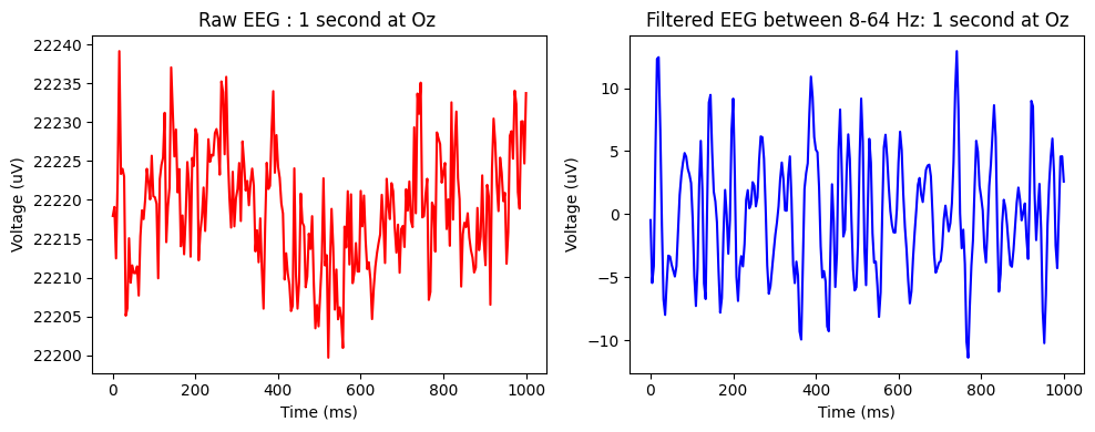
原始腦電圖 vs 濾波腦電圖 圖中說明了受試者 s1 在 Oz(視覺皮層的中央電極,頭部後方)記錄的相同 1 秒記錄。左側是記錄的原始腦電圖,右側是在 [8, 64] Hz 頻帶上濾波的腦電圖。我們看到較少的雜訊和自然腦電圖範圍內的正規化振幅值。
elec = 6  # Oz channel

x_label = "Time (ms)"
y_label = "Voltage (uV)"
# Create subplots
fig, (ax1, ax2) = plt.subplots(1, 2, figsize=(10, 4))

# Plot data on the first subplot
ax1.plot(time, X_raw[:, elec, 0, 0], "r-")
ax1.set_xlabel(x_label)
ax1.set_ylabel(y_label)
ax1.set_title("Raw EEG : 1 second at Oz ")

# Plot data on the second subplot
ax2.plot(time, X[0, :, elec, 0], "b-")
ax2.set_xlabel(x_label)
ax2.set_ylabel(y_label)
ax2.set_title("Filtered EEG between 8-64 Hz: 1 second at Oz")

# Adjust spacing between subplots
plt.tight_layout()

# Show the plot
plt.show()
腦電圖頻率表示
使用 Welch 方法,我們可視化表現良好的受試者在 Oz 電極上記錄的整個 4 秒腦電圖記錄的頻率功率,針對每個刺激。紅色峰值指示刺激的基頻和二次諧波(基頻的兩倍)。我們看到清晰的峰值,顯示該受試者的高響應,這表示該受試者是 SSVEP BCI 控制的良好候選人。在許多情況下,峰值很弱或不存在,表示受試者未正確完成任務。

建立層和模型
以跨框架自訂元件的方式建立層。在 SSVEPFormer 中,資料首先透過快速傅立葉轉換 (FFT) 轉換到頻域,以建構一個複雜的頻譜表示,其中包含固定頻帶中頻率和相位資訊的串連。為了保持模型以端對端格式,我們將複頻譜轉換實作為不可訓練層。
 SSVEPFormer 與 Transformer 架構不同,它不包含位置編碼/嵌入層,而是替換為通道組合區塊,該區塊具有一個卷積 1D 層,其核心大小為 1,濾波器數量是輸入通道(電極計數的兩倍)的兩倍,以及 LayerNorm、Gelu 激活和 dropout。與 Transformer 的另一個不同之處是缺少具有注意力機制的多頭注意力層。模型編碼器包含兩個相同的連續區塊。每個區塊都有兩個 CNN 模組和 MLP 模組的子區塊。CNN 模組包含 LayerNorm、卷積 1D(濾波器數量與通道組合相同)、LayerNorm、Gelu、Dropout 和殘差連接。MLP 模組包含 LayerNorm、密集層、Gelu、dropout 和殘差連接。密集層單獨應用於每個通道。模型的最後一個區塊是 MLP 頭部,包含 Flatten 層、Dropout、密集層、LayerNorm、Gelu、Dropout 和具有 softmax 激活的密集層。所有可訓練權重都透過平均值為 0 和標準差為 0.01 的常態分佈初始化,這與原始論文中的狀態相同。
class ComplexSpectrum(keras.layers.Layer):
    def __init__(self, nfft=512, fft_start=8, fft_end=64):
        super().__init__()
        self.nfft = nfft
        self.fft_start = fft_start
        self.fft_end = fft_end

    def call(self, x):
        samples = x.shape[-1]
        x = keras.ops.rfft(x, fft_length=self.nfft)
        real = x[0] / samples
        imag = x[1] / samples
        real = real[:, :, self.fft_start : self.fft_end]
        imag = imag[:, :, self.fft_start : self.fft_end]
        x = keras.ops.concatenate((real, imag), axis=-1)
        return x


class ChannelComb(keras.layers.Layer):
    def __init__(self, n_channels, drop_rate=0.5):
        super().__init__()
        self.conv = layers.Conv1D(
            2 * n_channels,
            1,
            padding="same",
            kernel_initializer=keras.initializers.RandomNormal(
                mean=0.0, stddev=0.01, seed=None
            ),
        )
        self.normalization = layers.LayerNormalization()
        self.activation = layers.Activation(activation="gelu")
        self.drop = layers.Dropout(drop_rate)

    def call(self, x):
        x = self.conv(x)
        x = self.normalization(x)
        x = self.activation(x)
        x = self.drop(x)
        return x


class ConvAttention(keras.layers.Layer):
    def __init__(self, n_channels, drop_rate=0.5):
        super().__init__()
        self.norm = layers.LayerNormalization()
        self.conv = layers.Conv1D(
            2 * n_channels,
            31,
            padding="same",
            kernel_initializer=keras.initializers.RandomNormal(
                mean=0.0, stddev=0.01, seed=None
            ),
        )
        self.activation = layers.Activation(activation="gelu")
        self.drop = layers.Dropout(drop_rate)

    def call(self, x):
        input = x
        x = self.norm(x)
        x = self.conv(x)
        x = self.activation(x)
        x = self.drop(x)
        x = x + input
        return x


class ChannelMLP(keras.layers.Layer):
    def __init__(self, n_features, drop_rate=0.5):
        super().__init__()
        self.norm = layers.LayerNormalization()
        self.mlp = layers.Dense(
            2 * n_features,
            kernel_initializer=keras.initializers.RandomNormal(
                mean=0.0, stddev=0.01, seed=None
            ),
        )
        self.activation = layers.Activation(activation="gelu")
        self.drop = layers.Dropout(drop_rate)
        self.cat = layers.Concatenate(axis=1)

    def call(self, x):
        input = x
        channels = x.shape[1]  # x shape : NCF
        x = self.norm(x)
        output_channels = []
        for i in range(channels):
            c = self.mlp(x[:, :, i])
            c = layers.Reshape([1, -1])(c)
            output_channels.append(c)
        x = self.cat(output_channels)
        x = self.activation(x)
        x = self.drop(x)
        x = x + input
        return x


class Encoder(keras.layers.Layer):
    def __init__(self, n_channels, n_features, drop_rate=0.5):
        super().__init__()
        self.attention1 = ConvAttention(n_channels, drop_rate=drop_rate)
        self.mlp1 = ChannelMLP(n_features, drop_rate=drop_rate)
        self.attention2 = ConvAttention(n_channels, drop_rate=drop_rate)
        self.mlp2 = ChannelMLP(n_features, drop_rate=drop_rate)

    def call(self, x):
        x = self.attention1(x)
        x = self.mlp1(x)
        x = self.attention2(x)
        x = self.mlp2(x)
        return x


class MlpHead(keras.layers.Layer):
    def __init__(self, n_classes, drop_rate=0.5):
        super().__init__()
        self.flatten = layers.Flatten()
        self.drop = layers.Dropout(drop_rate)
        self.linear1 = layers.Dense(
            6 * n_classes,
            kernel_initializer=keras.initializers.RandomNormal(
                mean=0.0, stddev=0.01, seed=None
            ),
        )
        self.norm = layers.LayerNormalization()
        self.activation = layers.Activation(activation="gelu")
        self.drop2 = layers.Dropout(drop_rate)
        self.linear2 = layers.Dense(
            n_classes,
            kernel_initializer=keras.initializers.RandomNormal(
                mean=0.0, stddev=0.01, seed=None
            ),
        )

    def call(self, x):
        x = self.flatten(x)
        x = self.drop(x)
        x = self.linear1(x)
        x = self.norm(x)
        x = self.activation(x)
        x = self.drop2(x)
        x = self.linear2(x)
        return x
使用以上層建立循序模型
def create_ssvepformer(
    input_shape, fs, resolution, fq_band, n_channels, n_classes, drop_rate
):
    nfft = round(fs / resolution)
    fft_start = int(fq_band[0] / resolution)
    fft_end = int(fq_band[1] / resolution) + 1
    n_features = fft_end - fft_start

    model = keras.Sequential(
        [
            keras.Input(shape=input_shape),
            ComplexSpectrum(nfft, fft_start, fft_end),
            ChannelComb(n_channels=n_channels, drop_rate=drop_rate),
            Encoder(n_channels=n_channels, n_features=n_features, drop_rate=drop_rate),
            Encoder(n_channels=n_channels, n_features=n_features, drop_rate=drop_rate),
            MlpHead(n_classes=n_classes, drop_rate=drop_rate),
            layers.Activation(activation="softmax"),
        ]
    )

    return model
評估
# Training settings same as the original paper
BATCH_SIZE = 128
EPOCHS = 100
LR = 0.001  # learning rate
WD = 0.001  # weight decay
MOMENTUM = 0.9
DROP_RATE = 0.5

resolution = 0.25
從整個資料集中,我們選擇用於每個受試者評估的摺疊。建構用於訓練和測試資料的 tf 資料集物件,並建立模型並使用 SGD 優化器啟動訓練。
def concatenate_subjects(x, y, fold):
    X = np.concatenate([x[idx] for idx in fold], axis=-1)
    Y = np.concatenate([y[idx] for idx in fold], axis=-1)
    X = X.transpose((2, 1, 0))  # trials x channels x samples
    return X, Y - 1  # transform labels to values from 0...11


def evaluate_subject(
    x_train,
    y_train,
    x_val,
    y_val,
    input_shape,
    fs=256,
    resolution=0.25,
    band=[8, 64],
    channels=8,
    n_classes=12,
    drop_rate=DROP_RATE,
):

    train_dataset = (
        tf.data.Dataset.from_tensor_slices((x_train, y_train))
        .batch(BATCH_SIZE)
        .prefetch(tf.data.AUTOTUNE)
    )

    test_dataset = (
        tf.data.Dataset.from_tensor_slices((x_val, y_val))
        .batch(BATCH_SIZE)
        .prefetch(tf.data.AUTOTUNE)
    )

    model = create_ssvepformer(
        input_shape, fs, resolution, band, channels, n_classes, drop_rate
    )
    sgd = keras.optimizers.SGD(learning_rate=LR, momentum=MOMENTUM, weight_decay=WD)

    model.compile(
        loss="sparse_categorical_crossentropy",
        optimizer=sgd,
        metrics=["accuracy"],
        jit_compile=True,
    )

    history = model.fit(
        train_dataset,
        batch_size=BATCH_SIZE,
        epochs=EPOCHS,
        validation_data=test_dataset,
        verbose=0,
    )
    loss, acc = model.evaluate(test_dataset)
    return acc * 100
執行評估
channels = X.shape[2]
samples = X.shape[1]
input_shape = (channels, samples)
n_classes = 12

model = create_ssvepformer(
    input_shape, fs, resolution, band, channels, n_classes, DROP_RATE
)
model.summary()
Model: "sequential"
┏━━━━━━━━━━━━━━━━━━━━━━━━━━━━━━━━━━━━━━┳━━━━━━━━━━━━━━━━━━━━━━━━━━━━━┳━━━━━━━━━━━━━━━━━┓
┃ Layer (type)                         ┃ Output Shape                ┃         Param # ┃
┡━━━━━━━━━━━━━━━━━━━━━━━━━━━━━━━━━━━━━━╇━━━━━━━━━━━━━━━━━━━━━━━━━━━━━╇━━━━━━━━━━━━━━━━━┩
│ complex_spectrum (ComplexSpectrum)   │ (None, 8, 450)              │               0 │
├──────────────────────────────────────┼─────────────────────────────┼─────────────────┤
│ channel_comb (ChannelComb)           │ (None, 16, 450)             │           1,044 │
├──────────────────────────────────────┼─────────────────────────────┼─────────────────┤
│ encoder (Encoder)                    │ (None, 16, 450)             │          34,804 │
├──────────────────────────────────────┼─────────────────────────────┼─────────────────┤
│ encoder_1 (Encoder)                  │ (None, 16, 450)             │          34,804 │
├──────────────────────────────────────┼─────────────────────────────┼─────────────────┤
│ mlp_head (MlpHead)                   │ (None, 12)                  │         519,492 │
├──────────────────────────────────────┼─────────────────────────────┼─────────────────┤
│ activation_10 (Activation)           │ (None, 12)                  │               0 │
└──────────────────────────────────────┴─────────────────────────────┴─────────────────┘
Total params: 590,144 (2.25 MB)
Trainable params: 590,144 (2.25 MB)
Non-trainable params: 0 (0.00 B)
在所有受試者上進行評估,遵循留一受試者交叉驗證資料劃分方案
accs = np.zeros(10)

for subject in range(10):
    print(f"Testing subject: {subject+ 1}")

    # create train / test folds
    folds = np.delete(np.arange(10), subject)
    train_index = folds
    test_index = [subject]

    # create data split for each subject
    x_train, y_train = concatenate_subjects(X, Y, train_index)
    x_val, y_val = concatenate_subjects(X, Y, test_index)

    # train and evaluate a fold and compute the time it takes
    acc = evaluate_subject(x_train, y_train, x_val, y_val, input_shape)

    accs[subject] = acc

print(f"\nAccuracy Across Subjects: {accs.mean()} % std: {np.std(accs)}")
Testing subject: 1

WARNING: All log messages before absl::InitializeLog() is called are written to STDERR
I0000 00:00:1737801392.665434    1425 cuda_executor.cc:1015] successful NUMA node read from SysFS had negative value (-1), but there must be at least one NUMA node, so returning NUMA node zero. See more at https://github.com/torvalds/linux/blob/v6.0/Documentation/ABI/testing/sysfs-bus-pci#L344-L355
I0000 00:00:1737801393.156241    1425 cuda_executor.cc:1015] successful NUMA node read from SysFS had negative value (-1), but there must be at least one NUMA node, so returning NUMA node zero. See more at https://github.com/torvalds/linux/blob/v6.0/Documentation/ABI/testing/sysfs-bus-pci#L344-L355
I0000 00:00:1737801393.156492    1425 cuda_executor.cc:1015] successful NUMA node read from SysFS had negative value (-1), but there must be at least one NUMA node, so returning NUMA node zero. See more at https://github.com/torvalds/linux/blob/v6.0/Documentation/ABI/testing/sysfs-bus-pci#L344-L355
I0000 00:00:1737801393.160002    1425 cuda_executor.cc:1015] successful NUMA node read from SysFS had negative value (-1), but there must be at least one NUMA node, so returning NUMA node zero. See more at https://github.com/torvalds/linux/blob/v6.0/Documentation/ABI/testing/sysfs-bus-pci#L344-L355
I0000 00:00:1737801393.160279    1425 cuda_executor.cc:1015] successful NUMA node read from SysFS had negative value (-1), but there must be at least one NUMA node, so returning NUMA node zero. See more at https://github.com/torvalds/linux/blob/v6.0/Documentation/ABI/testing/sysfs-bus-pci#L344-L355
I0000 00:00:1737801393.160421    1425 cuda_executor.cc:1015] successful NUMA node read from SysFS had negative value (-1), but there must be at least one NUMA node, so returning NUMA node zero. See more at https://github.com/torvalds/linux/blob/v6.0/Documentation/ABI/testing/sysfs-bus-pci#L344-L355
I0000 00:00:1737801393.168480    1425 cuda_executor.cc:1015] successful NUMA node read from SysFS had negative value (-1), but there must be at least one NUMA node, so returning NUMA node zero. See more at https://github.com/torvalds/linux/blob/v6.0/Documentation/ABI/testing/sysfs-bus-pci#L344-L355
I0000 00:00:1737801393.168667    1425 cuda_executor.cc:1015] successful NUMA node read from SysFS had negative value (-1), but there must be at least one NUMA node, so returning NUMA node zero. See more at https://github.com/torvalds/linux/blob/v6.0/Documentation/ABI/testing/sysfs-bus-pci#L344-L355
I0000 00:00:1737801393.168908    1425 cuda_executor.cc:1015] successful NUMA node read from SysFS had negative value (-1), but there must be at least one NUMA node, so returning NUMA node zero. See more at https://github.com/torvalds/linux/blob/v6.0/Documentation/ABI/testing/sysfs-bus-pci#L344-L355
1/2 ━━━━━━━━━━ [37m━━━━━━━━━━ 0 秒 7 毫秒/步 - 準確度:0.5938 - 損失:1.2483
2/2 ━━━━━━━━━━━━━━━━━━━━ 0 秒 39 毫秒/步 - 準確度:0.5868 - 損失:1.3010
Testing subject: 2
1/2 ━━━━━━━━━━[37m━━━━━━━━━━ 0 秒 7 毫秒/步 - 準確度:0.5469 - 損失:1.5270
2/2 ━━━━━━━━━━━━━━━━━━━━ 0 秒 7 毫秒/步 - 準確度:0.5119 - 損失:1.5974
Testing subject: 3
1/2 ━━━━━━━━━━[37m━━━━━━━━━━ 0 秒 7 毫秒/步 - 準確度:0.7266 - 損失:0.8867
2/2 ━━━━━━━━━━━━━━━━━━━━ 0 秒 7 毫秒/步 - 準確度:0.6903 - 損失:1.0117
Testing subject: 4
1/2 ━━━━━━━━━━[37m━━━━━━━━━━ 0 秒 7 毫秒/步 - 準確度:0.9688 - 損失:0.1574
2/2 ━━━━━━━━━━━━━━━━━━━━ 0 秒 8 毫秒/步 - 準確度:0.9637 - 損失:0.1487
Testing subject: 5
1/2 ━━━━━━━━━━[37m━━━━━━━━━━ 0 秒 7 毫秒/步 - 準確度:0.9375 - 損失:0.2184
2/2 ━━━━━━━━━━━━━━━━━━━━ 0 秒 7 毫秒/步 - 準確度:0.9458 - 損失:0.1887
Testing subject: 6
1/2 ━━━━━━━━━━[37m━━━━━━━━━━ 0 秒 12 毫秒/步 - 準確度:0.9688 - 損失:0.1117
2/2 ━━━━━━━━━━━━━━━━━━━━ 0 秒 10 毫秒/步 - 準確度:0.9674 - 損失:0.1018
Testing subject: 7
1/2 ━━━━━━━━━━[37m━━━━━━━━━━ 0 秒 7 毫秒/步 - 準確度:0.9141 - 損失:0.2639
2/2 ━━━━━━━━━━━━━━━━━━━━ 0 秒 7 毫秒/步 - 準確度:0.9158 - 損失:0.2592
Testing subject: 8
1/2 ━━━━━━━━━━[37m━━━━━━━━━━ 0 秒 9 毫秒/步 - 準確度:0.9922 - 損失:0.0562
2/2 ━━━━━━━━━━━━━━━━━━━━ 0 秒 20 毫秒/步 - 準確度:0.9937 - 損失:0.0518
Testing subject: 9
1/2 ━━━━━━━━━━[37m━━━━━━━━━━ 0 秒 7 毫秒/步 - 準確度:0.9844 - 損失:0.0669
2/2 ━━━━━━━━━━━━━━━━━━━━ 0 秒 8 毫秒/步 - 準確度:0.9837 - 損失:0.0701
Testing subject: 10
1/2 ━━━━━━━━━━[37m━━━━━━━━━━ 0 秒 10 毫秒/步 - 準確度:0.9219 - 損失:0.3438
2/2 ━━━━━━━━━━━━━━━━━━━━ 0 秒 18 毫秒/步 - 準確度:0.8999 - 損失:0.4543
Accuracy Across Subjects: 84.11111384630203 % std: 17.575586372993953
就這樣!我們看到一些在訓練集中沒有資料的受試者仍然可以達到幾乎 100% 的正確指令,而另一些受試者則表現不佳,準確度約為 50%。在原始論文中使用 PyTorch 時,平均準確度為 84.04%,標準差為 17.37%。考慮到深度學習的隨機性,我們達到了相同的數值。
可視化
在 Colab Free/Pro/Pro+ 提供的三種 GPU:T4、L4、A100 上,不同後端(Jax、Tensorflow 和 PyTorch)之間的訓練和推論時間比較。
訓練時間

推論時間

在所有 GPU 上,Jax 後端在訓練和推論方面都是最好的,PyTorch 極其緩慢,原因是 jit 編譯選項被停用,因為 FFT 計算的複數資料類型不受 PyTorch jit 編譯器支援。
致謝
感謝 Chris Perry X @GoogleColab 支援此 GPU 計算工作。
參考文獻
[1] Chen, J. 等人。(2023) ‘用於 SSVEP 分類的基於 Transformer 的深度神經網路模型’,《Neural Networks》,164,第 521–534 頁。網址:https://doi.org/10.1016/j.neunet.2023.04.045。
[2] Nakanishi, M. 等人。(2015) ‘用於偵測穩態視覺誘發電位的典型相關分析方法之比較研究’,《Plos One》,10(10),第 e0140703 頁。網址:https://doi.org/10.1371/journal.pone.0140703