使用圖神經網路與 LSTM 進行交通預測
作者: Arash Khodadadi
建立日期 2021/12/28
上次修改日期 2023/11/22
說明: 此範例示範如何對圖形進行時間序列預測。

簡介
此範例展示如何使用圖神經網路和 LSTM 預測交通狀況。具體來說,我們有興趣在已知一系列路段的交通速度歷史紀錄後,預測未來交通速度值。
解決此問題的一種常見方法是將每個路段的交通速度視為獨立的時間序列,並使用相同時間序列的過去值來預測每個時間序列的未來值。
然而,此方法忽略了一個路段的交通速度對相鄰路段的依賴性。為了能夠考慮到相鄰道路集合上交通速度之間複雜的相互作用,我們可以將交通網路定義為圖形,並將交通速度視為此圖形上的訊號。在此範例中,我們實作了一個神經網路架構,可以處理圖形上的時間序列資料。我們首先展示如何處理資料並建立用於圖形預測的 tf.data.Dataset。然後,我們實作一個模型,該模型使用圖形卷積和 LSTM 層來執行圖形預測。
資料處理和模型架構的靈感來自這篇論文
Yu, Bing, Haoteng Yin, and Zhanxing Zhu. "Spatio-temporal graph convolutional networks: a deep learning framework for traffic forecasting." Proceedings of the 27th International Joint Conference on Artificial Intelligence, 2018. (github)
設定
import os

os.environ["KERAS_BACKEND"] = "tensorflow"

import pandas as pd
import numpy as np
import typing
import matplotlib.pyplot as plt

import tensorflow as tf
import keras
from keras import layers
from keras import ops
資料準備
資料說明
我們使用名為 PeMSD7 的真實世界交通速度資料集。我們使用 Yu et al., 2018 收集和準備的版本,可在此處取得。
資料包含兩個檔案
PeMSD7_W_228.csv包含加州第 7 區 228 個站點之間的距離。PeMSD7_V_228.csv包含 2012 年 5 月和 6 月平日收集的這些站點的交通速度。
資料集的完整說明可以在 Yu et al., 2018 中找到。
載入資料
url = "https://github.com/VeritasYin/STGCN_IJCAI-18/raw/master/dataset/PeMSD7_Full.zip"
data_dir = keras.utils.get_file(origin=url, extract=True, archive_format="zip")
data_dir = data_dir.rstrip("PeMSD7_Full.zip")

route_distances = pd.read_csv(
    os.path.join(data_dir, "PeMSD7_W_228.csv"), header=None
).to_numpy()
speeds_array = pd.read_csv(
    os.path.join(data_dir, "PeMSD7_V_228.csv"), header=None
).to_numpy()

print(f"route_distances shape={route_distances.shape}")
print(f"speeds_array shape={speeds_array.shape}")
route_distances shape=(228, 228)
speeds_array shape=(12672, 228)
子採樣道路
為了縮減問題規模並加快訓練速度,我們將僅使用資料集中 228 條道路中的 26 條道路樣本。我們選擇道路的方式是從道路 0 開始,選擇與其最接近的 5 條道路,然後繼續此過程,直到獲得 25 條道路。您可以選擇道路的任何其他子集。我們以這種方式選擇道路,以增加擁有速度時間序列相關道路的可能性。sample_routes 包含選定道路的 ID。
sample_routes = [
    0,
    1,
    4,
    7,
    8,
    11,
    15,
    108,
    109,
    114,
    115,
    118,
    120,
    123,
    124,
    126,
    127,
    129,
    130,
    132,
    133,
    136,
    139,
    144,
    147,
    216,
]
route_distances = route_distances[np.ix_(sample_routes, sample_routes)]
speeds_array = speeds_array[:, sample_routes]

print(f"route_distances shape={route_distances.shape}")
print(f"speeds_array shape={speeds_array.shape}")
route_distances shape=(26, 26)
speeds_array shape=(12672, 26)
資料視覺化
以下是兩條路線的交通速度時間序列
plt.figure(figsize=(18, 6))
plt.plot(speeds_array[:, [0, -1]])
plt.legend(["route_0", "route_25"])
<matplotlib.legend.Legend at 0x7f5a870b2050>

我們也可以視覺化不同路線中時間序列之間的相關性。
plt.figure(figsize=(8, 8))
plt.matshow(np.corrcoef(speeds_array.T), 0)
plt.xlabel("road number")
plt.ylabel("road number")
Text(0, 0.5, 'road number')
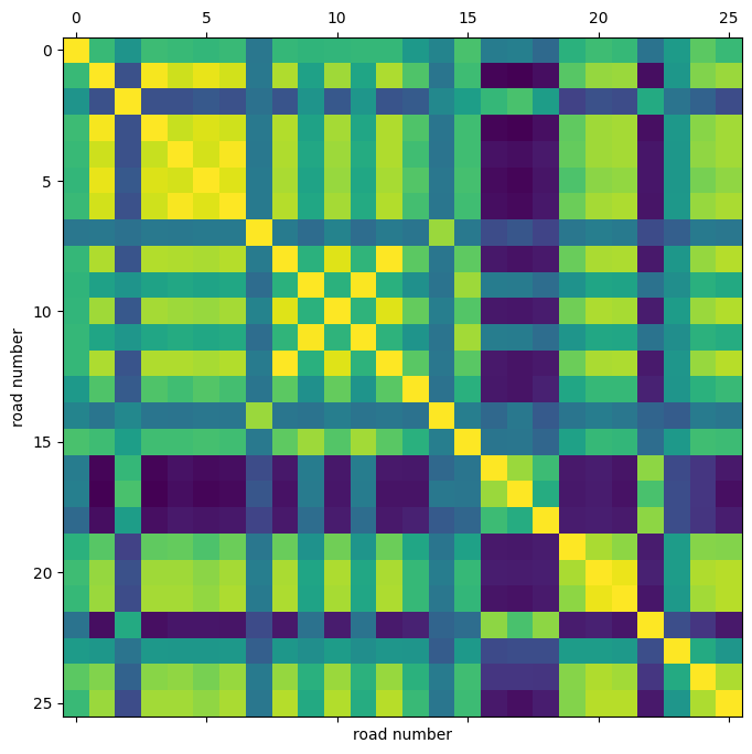
使用此相關性熱圖,我們可以觀察到,例如路線 4、5、6 的速度高度相關。
分割和正規化資料
接下來,我們將速度值陣列分割為訓練/驗證/測試集,並正規化產生的陣列
train_size, val_size = 0.5, 0.2


def preprocess(data_array: np.ndarray, train_size: float, val_size: float):
    """Splits data into train/val/test sets and normalizes the data.

    Args:
        data_array: ndarray of shape `(num_time_steps, num_routes)`
        train_size: A float value between 0.0 and 1.0 that represent the proportion of the dataset
            to include in the train split.
        val_size: A float value between 0.0 and 1.0 that represent the proportion of the dataset
            to include in the validation split.

    Returns:
        `train_array`, `val_array`, `test_array`
    """

    num_time_steps = data_array.shape[0]
    num_train, num_val = (
        int(num_time_steps * train_size),
        int(num_time_steps * val_size),
    )
    train_array = data_array[:num_train]
    mean, std = train_array.mean(axis=0), train_array.std(axis=0)

    train_array = (train_array - mean) / std
    val_array = (data_array[num_train : (num_train + num_val)] - mean) / std
    test_array = (data_array[(num_train + num_val) :] - mean) / std

    return train_array, val_array, test_array


train_array, val_array, test_array = preprocess(speeds_array, train_size, val_size)

print(f"train set size: {train_array.shape}")
print(f"validation set size: {val_array.shape}")
print(f"test set size: {test_array.shape}")
train set size: (6336, 26)
validation set size: (2534, 26)
test set size: (3802, 26)
建立 TensorFlow 資料集
接下來,我們為預測問題建立資料集。預測問題可以表述如下:給定時間 t+1, t+2, ..., t+T 的道路速度值序列,我們想要預測時間 t+T+1, ..., t+T+h 的未來道路速度值。因此,對於每個時間 t,我們模型的輸入是 T 個大小為 N 的向量,而目標是 h 個大小為 N 的向量,其中 N 是道路數量。
我們使用 Keras 內建函式 keras.utils.timeseries_dataset_from_array。函式 create_tf_dataset() 接收 numpy.ndarray 作為輸入,並傳回 tf.data.Dataset。在此函式中,input_sequence_length=T 且 forecast_horizon=h。
引數 multi_horizon 需要更多說明。假設 forecast_horizon=3。如果 multi_horizon=True,則模型將預測時間步長 t+T+1, t+T+2, t+T+3。因此,目標的形狀將為 (T,3)。但是,如果 multi_horizon=False,則模型將僅預測時間步長 t+T+3,因此目標的形狀將為 (T, 1)。
您可能會注意到,每個批次中的輸入張量形狀為 (batch_size, input_sequence_length, num_routes, 1)。新增最後一個維度是為了使模型更通用:在每個時間步長,每個道路的輸入特徵可能包含多個時間序列。例如,除了速度的歷史值之外,人們可能還想使用溫度時間序列作為輸入特徵。然而,在此範例中,輸入的最後一個維度始終為 1。
我們使用每條道路的最後 12 個速度值來預測未來 3 個時間步長的速度
batch_size = 64
input_sequence_length = 12
forecast_horizon = 3
multi_horizon = False


def create_tf_dataset(
    data_array: np.ndarray,
    input_sequence_length: int,
    forecast_horizon: int,
    batch_size: int = 128,
    shuffle=True,
    multi_horizon=True,
):
    """Creates tensorflow dataset from numpy array.

    This function creates a dataset where each element is a tuple `(inputs, targets)`.
    `inputs` is a Tensor
    of shape `(batch_size, input_sequence_length, num_routes, 1)` containing
    the `input_sequence_length` past values of the timeseries for each node.
    `targets` is a Tensor of shape `(batch_size, forecast_horizon, num_routes)`
    containing the `forecast_horizon`
    future values of the timeseries for each node.

    Args:
        data_array: np.ndarray with shape `(num_time_steps, num_routes)`
        input_sequence_length: Length of the input sequence (in number of timesteps).
        forecast_horizon: If `multi_horizon=True`, the target will be the values of the timeseries for 1 to
            `forecast_horizon` timesteps ahead. If `multi_horizon=False`, the target will be the value of the
            timeseries `forecast_horizon` steps ahead (only one value).
        batch_size: Number of timeseries samples in each batch.
        shuffle: Whether to shuffle output samples, or instead draw them in chronological order.
        multi_horizon: See `forecast_horizon`.

    Returns:
        A tf.data.Dataset instance.
    """

    inputs = keras.utils.timeseries_dataset_from_array(
        np.expand_dims(data_array[:-forecast_horizon], axis=-1),
        None,
        sequence_length=input_sequence_length,
        shuffle=False,
        batch_size=batch_size,
    )

    target_offset = (
        input_sequence_length
        if multi_horizon
        else input_sequence_length + forecast_horizon - 1
    )
    target_seq_length = forecast_horizon if multi_horizon else 1
    targets = keras.utils.timeseries_dataset_from_array(
        data_array[target_offset:],
        None,
        sequence_length=target_seq_length,
        shuffle=False,
        batch_size=batch_size,
    )

    dataset = tf.data.Dataset.zip((inputs, targets))
    if shuffle:
        dataset = dataset.shuffle(100)

    return dataset.prefetch(16).cache()


train_dataset, val_dataset = (
    create_tf_dataset(data_array, input_sequence_length, forecast_horizon, batch_size)
    for data_array in [train_array, val_array]
)

test_dataset = create_tf_dataset(
    test_array,
    input_sequence_length,
    forecast_horizon,
    batch_size=test_array.shape[0],
    shuffle=False,
    multi_horizon=multi_horizon,
)
道路圖形
如前所述,我們假設路段形成一個圖形。PeMSD7 資料集具有路段距離。下一步是從這些距離建立圖形鄰接矩陣。依照 Yu et al., 2018(方程式 10),我們假設如果對應道路之間的距離小於閾值,則圖形中兩個節點之間存在邊。
def compute_adjacency_matrix(
    route_distances: np.ndarray, sigma2: float, epsilon: float
):
    """Computes the adjacency matrix from distances matrix.

    It uses the formula in https://github.com/VeritasYin/STGCN_IJCAI-18#data-preprocessing to
    compute an adjacency matrix from the distance matrix.
    The implementation follows that paper.

    Args:
        route_distances: np.ndarray of shape `(num_routes, num_routes)`. Entry `i,j` of this array is the
            distance between roads `i,j`.
        sigma2: Determines the width of the Gaussian kernel applied to the square distances matrix.
        epsilon: A threshold specifying if there is an edge between two nodes. Specifically, `A[i,j]=1`
            if `np.exp(-w2[i,j] / sigma2) >= epsilon` and `A[i,j]=0` otherwise, where `A` is the adjacency
            matrix and `w2=route_distances * route_distances`

    Returns:
        A boolean graph adjacency matrix.
    """
    num_routes = route_distances.shape[0]
    route_distances = route_distances / 10000.0
    w2, w_mask = (
        route_distances * route_distances,
        np.ones([num_routes, num_routes]) - np.identity(num_routes),
    )
    return (np.exp(-w2 / sigma2) >= epsilon) * w_mask
函式 compute_adjacency_matrix() 傳回一個布林鄰接矩陣,其中 1 表示兩個節點之間存在邊。我們使用以下類別來儲存有關圖形的資訊。
class GraphInfo:
    def __init__(self, edges: typing.Tuple[list, list], num_nodes: int):
        self.edges = edges
        self.num_nodes = num_nodes


sigma2 = 0.1
epsilon = 0.5
adjacency_matrix = compute_adjacency_matrix(route_distances, sigma2, epsilon)
node_indices, neighbor_indices = np.where(adjacency_matrix == 1)
graph = GraphInfo(
    edges=(node_indices.tolist(), neighbor_indices.tolist()),
    num_nodes=adjacency_matrix.shape[0],
)
print(f"number of nodes: {graph.num_nodes}, number of edges: {len(graph.edges[0])}")
number of nodes: 26, number of edges: 150
網路架構
我們的圖形預測模型包含一個圖形卷積層和一個 LSTM 層。
圖形卷積層
我們對圖形卷積層的實作類似於 此 Keras 範例 中的實作。請注意,在該範例中,圖層的輸入是形狀為 (num_nodes,in_feat) 的 2D 張量,但在我們的範例中,圖層的輸入是形狀為 (num_nodes, batch_size, input_seq_length, in_feat) 的 4D 張量。圖形卷積層執行以下步驟
- 節點的表示在
self.compute_nodes_representation()中計算,方法是將輸入特徵乘以self.weight - 聚合的鄰居訊息在
self.compute_aggregated_messages()中計算,方法是首先聚合鄰居的表示,然後將結果乘以self.weight - 圖層的最終輸出在
self.update()中計算,方法是組合節點表示和鄰居的聚合訊息
class GraphConv(layers.Layer):
    def __init__(
        self,
        in_feat,
        out_feat,
        graph_info: GraphInfo,
        aggregation_type="mean",
        combination_type="concat",
        activation: typing.Optional[str] = None,
        **kwargs,
    ):
        super().__init__(**kwargs)
        self.in_feat = in_feat
        self.out_feat = out_feat
        self.graph_info = graph_info
        self.aggregation_type = aggregation_type
        self.combination_type = combination_type
        self.weight = self.add_weight(
            initializer=keras.initializers.GlorotUniform(),
            shape=(in_feat, out_feat),
            dtype="float32",
            trainable=True,
        )
        self.activation = layers.Activation(activation)

    def aggregate(self, neighbour_representations):
        aggregation_func = {
            "sum": tf.math.unsorted_segment_sum,
            "mean": tf.math.unsorted_segment_mean,
            "max": tf.math.unsorted_segment_max,
        }.get(self.aggregation_type)

        if aggregation_func:
            return aggregation_func(
                neighbour_representations,
                self.graph_info.edges[0],
                num_segments=self.graph_info.num_nodes,
            )

        raise ValueError(f"Invalid aggregation type: {self.aggregation_type}")

    def compute_nodes_representation(self, features):
        """Computes each node's representation.

        The nodes' representations are obtained by multiplying the features tensor with
        `self.weight`. Note that
        `self.weight` has shape `(in_feat, out_feat)`.

        Args:
            features: Tensor of shape `(num_nodes, batch_size, input_seq_len, in_feat)`

        Returns:
            A tensor of shape `(num_nodes, batch_size, input_seq_len, out_feat)`
        """
        return ops.matmul(features, self.weight)

    def compute_aggregated_messages(self, features):
        neighbour_representations = tf.gather(features, self.graph_info.edges[1])
        aggregated_messages = self.aggregate(neighbour_representations)
        return ops.matmul(aggregated_messages, self.weight)

    def update(self, nodes_representation, aggregated_messages):
        if self.combination_type == "concat":
            h = ops.concatenate([nodes_representation, aggregated_messages], axis=-1)
        elif self.combination_type == "add":
            h = nodes_representation + aggregated_messages
        else:
            raise ValueError(f"Invalid combination type: {self.combination_type}.")
        return self.activation(h)

    def call(self, features):
        """Forward pass.

        Args:
            features: tensor of shape `(num_nodes, batch_size, input_seq_len, in_feat)`

        Returns:
            A tensor of shape `(num_nodes, batch_size, input_seq_len, out_feat)`
        """
        nodes_representation = self.compute_nodes_representation(features)
        aggregated_messages = self.compute_aggregated_messages(features)
        return self.update(nodes_representation, aggregated_messages)
LSTM 加圖形卷積
透過將圖形卷積層應用於輸入張量,我們獲得另一個包含節點隨時間推移的表示的張量(另一個 4D 張量)。對於每個時間步長,節點的表示都會受到來自其鄰居的資訊的影響。
然而,為了做出良好的預測,我們不僅需要來自鄰居的資訊,還需要隨時間處理資訊。為此,我們可以將每個節點的張量傳遞到循環層。下面的 LSTMGC 層首先將圖形卷積層應用於輸入,然後將結果傳遞到 LSTM 層。
class LSTMGC(layers.Layer):
    """Layer comprising a convolution layer followed by LSTM and dense layers."""

    def __init__(
        self,
        in_feat,
        out_feat,
        lstm_units: int,
        input_seq_len: int,
        output_seq_len: int,
        graph_info: GraphInfo,
        graph_conv_params: typing.Optional[dict] = None,
        **kwargs,
    ):
        super().__init__(**kwargs)

        # graph conv layer
        if graph_conv_params is None:
            graph_conv_params = {
                "aggregation_type": "mean",
                "combination_type": "concat",
                "activation": None,
            }
        self.graph_conv = GraphConv(in_feat, out_feat, graph_info, **graph_conv_params)

        self.lstm = layers.LSTM(lstm_units, activation="relu")
        self.dense = layers.Dense(output_seq_len)

        self.input_seq_len, self.output_seq_len = input_seq_len, output_seq_len

    def call(self, inputs):
        """Forward pass.

        Args:
            inputs: tensor of shape `(batch_size, input_seq_len, num_nodes, in_feat)`

        Returns:
            A tensor of shape `(batch_size, output_seq_len, num_nodes)`.
        """

        # convert shape to  (num_nodes, batch_size, input_seq_len, in_feat)
        inputs = ops.transpose(inputs, [2, 0, 1, 3])

        gcn_out = self.graph_conv(
            inputs
        )  # gcn_out has shape: (num_nodes, batch_size, input_seq_len, out_feat)
        shape = ops.shape(gcn_out)
        num_nodes, batch_size, input_seq_len, out_feat = (
            shape[0],
            shape[1],
            shape[2],
            shape[3],
        )

        # LSTM takes only 3D tensors as input
        gcn_out = ops.reshape(
            gcn_out, (batch_size * num_nodes, input_seq_len, out_feat)
        )
        lstm_out = self.lstm(
            gcn_out
        )  # lstm_out has shape: (batch_size * num_nodes, lstm_units)

        dense_output = self.dense(
            lstm_out
        )  # dense_output has shape: (batch_size * num_nodes, output_seq_len)
        output = ops.reshape(dense_output, (num_nodes, batch_size, self.output_seq_len))
        return ops.transpose(
            output, [1, 2, 0]
        )  # returns Tensor of shape (batch_size, output_seq_len, num_nodes)
模型訓練
in_feat = 1
batch_size = 64
epochs = 20
input_sequence_length = 12
forecast_horizon = 3
multi_horizon = False
out_feat = 10
lstm_units = 64
graph_conv_params = {
    "aggregation_type": "mean",
    "combination_type": "concat",
    "activation": None,
}

st_gcn = LSTMGC(
    in_feat,
    out_feat,
    lstm_units,
    input_sequence_length,
    forecast_horizon,
    graph,
    graph_conv_params,
)
inputs = layers.Input((input_sequence_length, graph.num_nodes, in_feat))
outputs = st_gcn(inputs)

model = keras.models.Model(inputs, outputs)
model.compile(
    optimizer=keras.optimizers.RMSprop(learning_rate=0.0002),
    loss=keras.losses.MeanSquaredError(),
)
model.fit(
    train_dataset,
    validation_data=val_dataset,
    epochs=epochs,
    callbacks=[keras.callbacks.EarlyStopping(patience=10)],
)
Epoch 1/20
1/99 [37m━━━━━━━━━━━━━━━━━━━━ 5:16 3s/step - loss: 1.0735
WARNING: All log messages before absl::InitializeLog() is called are written to STDERR
I0000 00:00:1700705896.341813 3354152 device_compiler.h:186] Compiled cluster using XLA! This line is logged at most once for the lifetime of the process.
W0000 00:00:1700705896.362213 3354152 graph_launch.cc:671] Fallback to op-by-op mode because memset node breaks graph update
W0000 00:00:1700705896.363019 3354152 graph_launch.cc:671] Fallback to op-by-op mode because memset node breaks graph update
44/99 ━━━━━━━━[37m━━━━━━━━━━━━ 1s 32ms/step - loss: 0.7919
W0000 00:00:1700705897.577991 3354154 graph_launch.cc:671] Fallback to op-by-op mode because memset node breaks graph update
W0000 00:00:1700705897.578802 3354154 graph_launch.cc:671] Fallback to op-by-op mode because memset node breaks graph update
99/99 ━━━━━━━━━━━━━━━━━━━━ 7s 36ms/step - loss: 0.7470 - val_loss: 0.3568
Epoch 2/20
99/99 ━━━━━━━━━━━━━━━━━━━━ 0s 5ms/step - loss: 0.2785 - val_loss: 0.1845
Epoch 3/20
99/99 ━━━━━━━━━━━━━━━━━━━━ 0s 5ms/step - loss: 0.1734 - val_loss: 0.1250
Epoch 4/20
99/99 ━━━━━━━━━━━━━━━━━━━━ 0s 5ms/step - loss: 0.1313 - val_loss: 0.1084
Epoch 5/20
99/99 ━━━━━━━━━━━━━━━━━━━━ 0s 5ms/step - loss: 0.1095 - val_loss: 0.0994
Epoch 6/20
99/99 ━━━━━━━━━━━━━━━━━━━━ 0s 5ms/step - loss: 0.0960 - val_loss: 0.0930
Epoch 7/20
99/99 ━━━━━━━━━━━━━━━━━━━━ 0s 5ms/step - loss: 0.0896 - val_loss: 0.0954
Epoch 8/20
99/99 ━━━━━━━━━━━━━━━━━━━━ 0s 5ms/step - loss: 0.0862 - val_loss: 0.0920
Epoch 9/20
99/99 ━━━━━━━━━━━━━━━━━━━━ 1s 5ms/step - loss: 0.0841 - val_loss: 0.0898
Epoch 10/20
99/99 ━━━━━━━━━━━━━━━━━━━━ 1s 5ms/step - loss: 0.0827 - val_loss: 0.0884
Epoch 11/20
99/99 ━━━━━━━━━━━━━━━━━━━━ 1s 5ms/step - loss: 0.0817 - val_loss: 0.0865
Epoch 12/20
99/99 ━━━━━━━━━━━━━━━━━━━━ 0s 5ms/step - loss: 0.0809 - val_loss: 0.0843
Epoch 13/20
99/99 ━━━━━━━━━━━━━━━━━━━━ 0s 5ms/step - loss: 0.0803 - val_loss: 0.0828
Epoch 14/20
99/99 ━━━━━━━━━━━━━━━━━━━━ 0s 5ms/step - loss: 0.0798 - val_loss: 0.0814
Epoch 15/20
99/99 ━━━━━━━━━━━━━━━━━━━━ 0s 5ms/step - loss: 0.0794 - val_loss: 0.0802
Epoch 16/20
99/99 ━━━━━━━━━━━━━━━━━━━━ 0s 5ms/step - loss: 0.0790 - val_loss: 0.0794
Epoch 17/20
99/99 ━━━━━━━━━━━━━━━━━━━━ 0s 5ms/step - loss: 0.0787 - val_loss: 0.0786
Epoch 18/20
99/99 ━━━━━━━━━━━━━━━━━━━━ 0s 5ms/step - loss: 0.0785 - val_loss: 0.0780
Epoch 19/20
99/99 ━━━━━━━━━━━━━━━━━━━━ 0s 5ms/step - loss: 0.0782 - val_loss: 0.0776
Epoch 20/20
99/99 ━━━━━━━━━━━━━━━━━━━━ 0s 5ms/step - loss: 0.0780 - val_loss: 0.0776
<keras.src.callbacks.history.History at 0x7f59b8152560>
在測試集上進行預測
現在我們可以使用訓練好的模型對測試集進行預測。下面,我們計算模型的 MAE,並將其與樸素預測的 MAE 進行比較。樸素預測是每個節點速度的最後一個值。
x_test, y = next(test_dataset.as_numpy_iterator())
y_pred = model.predict(x_test)
plt.figure(figsize=(18, 6))
plt.plot(y[:, 0, 0])
plt.plot(y_pred[:, 0, 0])
plt.legend(["actual", "forecast"])

naive_mse, model_mse = (
    np.square(x_test[:, -1, :, 0] - y[:, 0, :]).mean(),
    np.square(y_pred[:, 0, :] - y[:, 0, :]).mean(),
)
print(f"naive MAE: {naive_mse}, model MAE: {model_mse}")
 119/119 ━━━━━━━━━━━━━━━━━━━━ 1s 6ms/step
naive MAE: 0.13472308593195767, model MAE: 0.13524348477186485
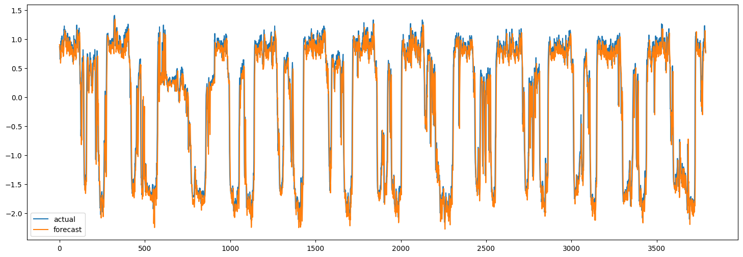
當然,這裡的目標是示範方法,而不是實現最佳效能。為了提高模型的準確性,應仔細調整所有模型超參數。此外,可以堆疊多個 LSTMGC 區塊以提高模型的表示能力。