► 程式碼範例 / 電腦視覺 / 使用 BigTransfer (BiT) 進行影像分類

使用 BigTransfer (BiT) 進行影像分類

作者： Sayan Nath
建立日期 2021/09/24
上次修改日期 2024/01/03
描述： BigTransfer (BiT) 用於影像分類的最新遷移學習。

ⓘ 這個範例使用 Keras 3

簡介

BigTransfer（也稱為 BiT）是一種用於影像分類的最新遷移學習方法。當訓練用於視覺的深度神經網路時，遷移預訓練表示可提高樣本效率並簡化超參數調整。BiT 重新檢視在大型監督資料集上預訓練，並在目標任務上微調模型的範式。適當選擇正規化層，並隨著預訓練資料量的增加而縮放架構容量的重要性。

BigTransfer (BiT) 是在公開資料集上訓練的，程式碼位於 TF2、Jax 和 Pytorch 中。這將幫助任何人達到他們感興趣任務的最新效能，即使每個類別只有少數標記的影像也是如此。

您可以在 TFHub 中找到在 ImageNet 和 ImageNet-21k 上預訓練的 BiT 模型，這些模型是 TensorFlow2 SavedModels，您可以輕鬆地將其用作 Keras 圖層。有多種尺寸可供選擇，從標準的 ResNet50 到 ResNet152x4（152 層深，比典型的 ResNet50 寬 4 倍），適用於具有較大計算和記憶體預算但對準確性有更高要求的用戶。

圖：x 軸顯示每個類別使用的影像數量，範圍從 1 到完整資料集。在左側的圖中，藍色上方的曲線是我們的 BiT-L 模型，而下方的曲線是在 ImageNet (ILSVRC-2012) 上預訓練的 ResNet-50。

設定

import os
os.environ["KERAS_BACKEND"] = "tensorflow"
import numpy as np
import pandas as pd
import matplotlib.pyplot as plt

import keras
from keras import ops
import tensorflow as tf
import tensorflow_hub as hub
import tensorflow_datasets as tfds

tfds.disable_progress_bar()

SEEDS = 42

keras.utils.set_random_seed(SEEDS)

收集花朵資料集

train_ds, validation_ds = tfds.load(
    "tf_flowers",
    split=["train[:85%]", "train[85%:]"],
    as_supervised=True,
)

[1mDownloading and preparing dataset 218.21 MiB (download: 218.21 MiB, generated: 221.83 MiB, total: 440.05 MiB) to ~/tensorflow_datasets/tf_flowers/3.0.1...[0m
[1mDataset tf_flowers downloaded and prepared to ~/tensorflow_datasets/tf_flowers/3.0.1. Subsequent calls will reuse this data.[0m

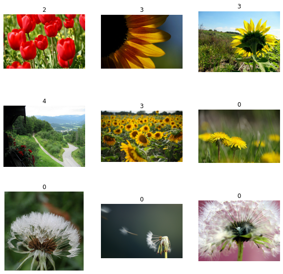
視覺化資料集

plt.figure(figsize=(10, 10))
for i, (image, label) in enumerate(train_ds.take(9)):
    ax = plt.subplot(3, 3, i + 1)
    plt.imshow(image)
    plt.title(int(label))
    plt.axis("off")

png

定義超參數

RESIZE_TO = 384
CROP_TO = 224
BATCH_SIZE = 64
STEPS_PER_EPOCH = 10
AUTO = tf.data.AUTOTUNE  # optimise the pipeline performance
NUM_CLASSES = 5  # number of classes
SCHEDULE_LENGTH = (
    500  # we will train on lower resolution images and will still attain good results
)
SCHEDULE_BOUNDARIES = [
    200,
    300,
    400,
]  # more the dataset size the schedule length increase

SCHEDULE_LENGTH 和 SCHEDULE_BOUNDARIES 等超參數是根據經驗結果確定的。該方法已在原始論文和他們的 Google AI 網誌文章中進行了解釋。

SCHEDULE_LENGTH 也決定是否要使用 MixUp 增強。您也可以在 Keras 程式碼範例中找到簡單的 MixUp 實作。

定義預處理輔助函數

SCHEDULE_LENGTH = SCHEDULE_LENGTH * 512 / BATCH_SIZE

random_flip = keras.layers.RandomFlip("horizontal")
random_crop = keras.layers.RandomCrop(CROP_TO, CROP_TO)

def preprocess_train(image, label):
    image = random_flip(image)
    image = ops.image.resize(image, (RESIZE_TO, RESIZE_TO))
    image = random_crop(image)
    image = image / 255.0
    return (image, label)


def preprocess_test(image, label):
    image = ops.image.resize(image, (RESIZE_TO, RESIZE_TO))
    image = ops.cast(image, dtype="float32")
    image = image / 255.0
    return (image, label)


DATASET_NUM_TRAIN_EXAMPLES = train_ds.cardinality().numpy()

repeat_count = int(
    SCHEDULE_LENGTH * BATCH_SIZE / DATASET_NUM_TRAIN_EXAMPLES * STEPS_PER_EPOCH
)
repeat_count += 50 + 1  # To ensure at least there are 50 epochs of training

定義資料管線

# Training pipeline
pipeline_train = (
    train_ds.shuffle(10000)
    .repeat(repeat_count)  # Repeat dataset_size / num_steps
    .map(preprocess_train, num_parallel_calls=AUTO)
    .batch(BATCH_SIZE)
    .prefetch(AUTO)
)

# Validation pipeline
pipeline_validation = (
    validation_ds.map(preprocess_test, num_parallel_calls=AUTO)
    .batch(BATCH_SIZE)
    .prefetch(AUTO)
)

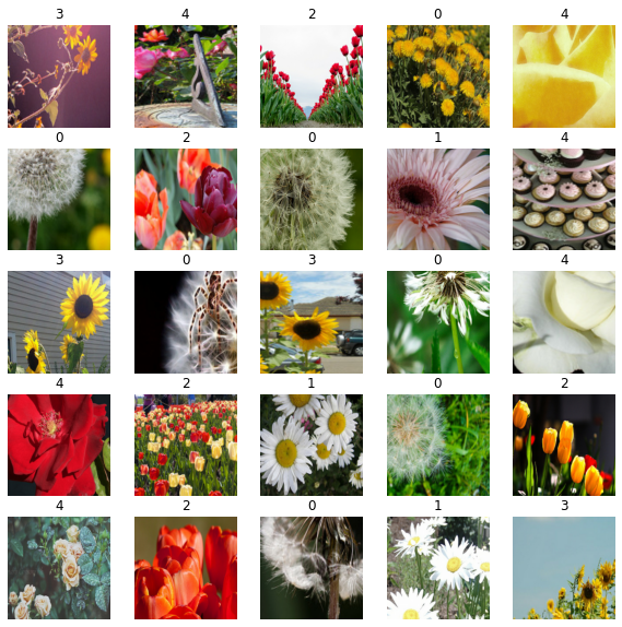
視覺化訓練樣本

image_batch, label_batch = next(iter(pipeline_train))

plt.figure(figsize=(10, 10))
for n in range(25):
    ax = plt.subplot(5, 5, n + 1)
    plt.imshow(image_batch[n])
    plt.title(label_batch[n].numpy())
    plt.axis("off")

png

將預訓練的 TF-Hub 模型載入到 `KerasLayer` 中

bit_model_url = "https://tfhub.dev/google/bit/m-r50x1/1"
bit_module = hub.load(bit_model_url)

建立 BigTransfer (BiT) 模型

要建立新模型，我們

切斷 BiT 模型原有的頭部。這會留下「預邏輯」輸出。如果我們使用「特徵提取器」模型（即子目錄中所有標題為 feature_vectors 的模型），則我們不必這樣做，因為對於這些模型，頭部已經被切斷。
新增一個新的頭部，其輸出數量等於我們新任務的類別數量。請注意，將頭部初始化為全零很重要。

class MyBiTModel(keras.Model):
    def __init__(self, num_classes, module, **kwargs):
        super().__init__(**kwargs)

        self.num_classes = num_classes
        self.head = keras.layers.Dense(num_classes, kernel_initializer="zeros")
        self.bit_model = module

    def call(self, images):
        bit_embedding = self.bit_model(images)
        return self.head(bit_embedding)


model = MyBiTModel(num_classes=NUM_CLASSES, module=bit_module)

定義最佳化器和損失

learning_rate = 0.003 * BATCH_SIZE / 512

# Decay learning rate by a factor of 10 at SCHEDULE_BOUNDARIES.
lr_schedule = keras.optimizers.schedules.PiecewiseConstantDecay(
    boundaries=SCHEDULE_BOUNDARIES,
    values=[
        learning_rate,
        learning_rate * 0.1,
        learning_rate * 0.01,
        learning_rate * 0.001,
    ],
)
optimizer = keras.optimizers.SGD(learning_rate=lr_schedule, momentum=0.9)

loss_fn = keras.losses.SparseCategoricalCrossentropy(from_logits=True)

編譯模型

model.compile(optimizer=optimizer, loss=loss_fn, metrics=["accuracy"])

設定回呼

train_callbacks = [
    keras.callbacks.EarlyStopping(
        monitor="val_accuracy", patience=2, restore_best_weights=True
    )
]

訓練模型

history = model.fit(
    pipeline_train,
    batch_size=BATCH_SIZE,
    epochs=int(SCHEDULE_LENGTH / STEPS_PER_EPOCH),
    steps_per_epoch=STEPS_PER_EPOCH,
    validation_data=pipeline_validation,
    callbacks=train_callbacks,
)

Epoch 1/400
10/10 [==============================] - 18s 852ms/step - loss: 0.7465 - accuracy: 0.7891 - val_loss: 0.1865 - val_accuracy: 0.9582
Epoch 2/400
10/10 [==============================] - 5s 529ms/step - loss: 0.1389 - accuracy: 0.9578 - val_loss: 0.1075 - val_accuracy: 0.9727
Epoch 3/400
10/10 [==============================] - 5s 520ms/step - loss: 0.1720 - accuracy: 0.9391 - val_loss: 0.0858 - val_accuracy: 0.9727
Epoch 4/400
10/10 [==============================] - 5s 525ms/step - loss: 0.1211 - accuracy: 0.9516 - val_loss: 0.0833 - val_accuracy: 0.9691

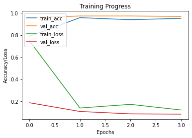
繪製訓練和驗證指標

def plot_hist(hist):
    plt.plot(hist.history["accuracy"])
    plt.plot(hist.history["val_accuracy"])
    plt.plot(hist.history["loss"])
    plt.plot(hist.history["val_loss"])
    plt.title("Training Progress")
    plt.ylabel("Accuracy/Loss")
    plt.xlabel("Epochs")
    plt.legend(["train_acc", "val_acc", "train_loss", "val_loss"], loc="upper left")
    plt.show()


plot_hist(history)

png

評估模型

accuracy = model.evaluate(pipeline_validation)[1] * 100
print("Accuracy: {:.2f}%".format(accuracy))

9/9 [==============================] - 3s 364ms/step - loss: 0.1075 - accuracy: 0.9727
Accuracy: 97.27%

結論

BiT 在驚人廣泛的資料範疇中表現良好 – 從每個類別 1 個範例到總共 100 萬個範例。BiT 在 ILSVRC-2012 上達到 87.5% 的前 1 準確度，在 CIFAR-10 上達到 99.4%，在 19 個任務視覺任務適應基準 (VTAB) 上達到 76.3%。在小型資料集上，BiT 在每個類別有 10 個範例的情況下在 ILSVRC-2012 上達到 76.8%，在每個類別有 10 個範例的情況下在 CIFAR-10 上達到 97.0%。