緊湊型卷積變換器
作者: Sayak Paul
建立日期 2021/06/30
上次修改日期 2023/08/07
描述: 用於高效圖像分類的緊湊型卷積變換器。

如 視覺變換器 (ViT) 論文中所討論的,用於視覺的基於變換器的架構通常需要比平常更大的資料集,以及更長的預訓練排程。ImageNet-1k (約有一百萬張圖像) 被認為在 ViT 方面屬於中型資料範圍。這主要是因為,與 CNN 不同,ViT (或典型的基於變換器的架構) 沒有充分了解的歸納偏置 (例如用於處理圖像的卷積)。這引發了一個問題:我們是否可以在單個網路架構中結合卷積的優點和變換器的優點?這些優點包括參數效率,以及用於處理長程和全域依賴關係 (圖像中不同區域之間的互動) 的自注意力。
在 使用緊湊型變換器擺脫大數據範式 中,Hassani 等人提出了一種完全實現此目標的方法。他們提出了緊湊型卷積變換器 (CCT) 架構。在此範例中,我們將著手實作 CCT,並了解它在 CIFAR-10 資料集上的效能如何。
如果您不熟悉自注意力或變換器的概念,可以閱讀 François Chollet 的書《使用 Python 進行深度學習》中的此章節。此範例使用另一個範例中的程式碼片段,使用視覺變換器進行圖像分類。
導入
from keras import layers
import keras

import matplotlib.pyplot as plt
import numpy as np
超參數和常數
positional_emb = True
conv_layers = 2
projection_dim = 128

num_heads = 2
transformer_units = [
    projection_dim,
    projection_dim,
]
transformer_layers = 2
stochastic_depth_rate = 0.1

learning_rate = 0.001
weight_decay = 0.0001
batch_size = 128
num_epochs = 30
image_size = 32
載入 CIFAR-10 資料集
num_classes = 10
input_shape = (32, 32, 3)

(x_train, y_train), (x_test, y_test) = keras.datasets.cifar10.load_data()

y_train = keras.utils.to_categorical(y_train, num_classes)
y_test = keras.utils.to_categorical(y_test, num_classes)

print(f"x_train shape: {x_train.shape} - y_train shape: {y_train.shape}")
print(f"x_test shape: {x_test.shape} - y_test shape: {y_test.shape}")
x_train shape: (50000, 32, 32, 3) - y_train shape: (50000, 10)
x_test shape: (10000, 32, 32, 3) - y_test shape: (10000, 10)
CCT 標記器
CCT 作者引入的第一個方法是用於處理圖像的標記器。在標準的 ViT 中,圖像被組織成統一的不重疊區塊。這消除了不同區塊之間存在的邊界層級資訊。這對於神經網路有效利用局部資訊非常重要。下圖說明了如何將圖像組織成區塊。

我們已經知道卷積非常擅長利用局部資訊。因此,基於此,作者引入了一個全卷積迷你網路來產生圖像區塊。
class CCTTokenizer(layers.Layer):
    def __init__(
        self,
        kernel_size=3,
        stride=1,
        padding=1,
        pooling_kernel_size=3,
        pooling_stride=2,
        num_conv_layers=conv_layers,
        num_output_channels=[64, 128],
        positional_emb=positional_emb,
        **kwargs,
    ):
        super().__init__(**kwargs)

        # This is our tokenizer.
        self.conv_model = keras.Sequential()
        for i in range(num_conv_layers):
            self.conv_model.add(
                layers.Conv2D(
                    num_output_channels[i],
                    kernel_size,
                    stride,
                    padding="valid",
                    use_bias=False,
                    activation="relu",
                    kernel_initializer="he_normal",
                )
            )
            self.conv_model.add(layers.ZeroPadding2D(padding))
            self.conv_model.add(
                layers.MaxPooling2D(pooling_kernel_size, pooling_stride, "same")
            )

        self.positional_emb = positional_emb

    def call(self, images):
        outputs = self.conv_model(images)
        # After passing the images through our mini-network the spatial dimensions
        # are flattened to form sequences.
        reshaped = keras.ops.reshape(
            outputs,
            (
                -1,
                keras.ops.shape(outputs)[1] * keras.ops.shape(outputs)[2],
                keras.ops.shape(outputs)[-1],
            ),
        )
        return reshaped
位置嵌入在 CCT 中是可選的。如果我們想使用它們,可以使用下面定義的層。
class PositionEmbedding(keras.layers.Layer):
    def __init__(
        self,
        sequence_length,
        initializer="glorot_uniform",
        **kwargs,
    ):
        super().__init__(**kwargs)
        if sequence_length is None:
            raise ValueError("`sequence_length` must be an Integer, received `None`.")
        self.sequence_length = int(sequence_length)
        self.initializer = keras.initializers.get(initializer)

    def get_config(self):
        config = super().get_config()
        config.update(
            {
                "sequence_length": self.sequence_length,
                "initializer": keras.initializers.serialize(self.initializer),
            }
        )
        return config

    def build(self, input_shape):
        feature_size = input_shape[-1]
        self.position_embeddings = self.add_weight(
            name="embeddings",
            shape=[self.sequence_length, feature_size],
            initializer=self.initializer,
            trainable=True,
        )

        super().build(input_shape)

    def call(self, inputs, start_index=0):
        shape = keras.ops.shape(inputs)
        feature_length = shape[-1]
        sequence_length = shape[-2]
        # trim to match the length of the input sequence, which might be less
        # than the sequence_length of the layer.
        position_embeddings = keras.ops.convert_to_tensor(self.position_embeddings)
        position_embeddings = keras.ops.slice(
            position_embeddings,
            (start_index, 0),
            (sequence_length, feature_length),
        )
        return keras.ops.broadcast_to(position_embeddings, shape)

    def compute_output_shape(self, input_shape):
        return input_shape
序列池化
CCT 中引入的另一個方法是注意力池化或序列池化。在 ViT 中,只有對應於類別權杖的特徵圖會被池化,然後用於後續的分類任務 (或任何其他下游任務)。
class SequencePooling(layers.Layer):
    def __init__(self):
        super().__init__()
        self.attention = layers.Dense(1)

    def call(self, x):
        attention_weights = keras.ops.softmax(self.attention(x), axis=1)
        attention_weights = keras.ops.transpose(attention_weights, axes=(0, 2, 1))
        weighted_representation = keras.ops.matmul(attention_weights, x)
        return keras.ops.squeeze(weighted_representation, -2)
用於正規化的隨機深度
隨機深度是一種隨機捨棄一組層的正規化技術。在推論期間,這些層會保持原樣。它與 Dropout 非常相似,但它只作用於一組層,而不是作用於層內存在的個別節點。在 CCT 中,隨機深度會用在變換器編碼器的殘差區塊之前。
# Referred from: github.com:rwightman/pytorch-image-models.
class StochasticDepth(layers.Layer):
    def __init__(self, drop_prop, **kwargs):
        super().__init__(**kwargs)
        self.drop_prob = drop_prop
        self.seed_generator = keras.random.SeedGenerator(1337)

    def call(self, x, training=None):
        if training:
            keep_prob = 1 - self.drop_prob
            shape = (keras.ops.shape(x)[0],) + (1,) * (len(x.shape) - 1)
            random_tensor = keep_prob + keras.random.uniform(
                shape, 0, 1, seed=self.seed_generator
            )
            random_tensor = keras.ops.floor(random_tensor)
            return (x / keep_prob) * random_tensor
        return x
用於變換器編碼器的 MLP
def mlp(x, hidden_units, dropout_rate):
    for units in hidden_units:
        x = layers.Dense(units, activation=keras.ops.gelu)(x)
        x = layers.Dropout(dropout_rate)(x)
    return x
資料擴增
在原始論文中,作者使用AutoAugment來誘導更強的正規化。在此範例中,我們將使用標準的幾何擴增,例如隨機裁剪和翻轉。
# Note the rescaling layer. These layers have pre-defined inference behavior.
data_augmentation = keras.Sequential(
    [
        layers.Rescaling(scale=1.0 / 255),
        layers.RandomCrop(image_size, image_size),
        layers.RandomFlip("horizontal"),
    ],
    name="data_augmentation",
)
最終的 CCT 模型
在 CCT 中,變換器編碼器的輸出會被加權,然後傳遞到最終的任務特定層 (在此範例中,我們執行分類)。
def create_cct_model(
    image_size=image_size,
    input_shape=input_shape,
    num_heads=num_heads,
    projection_dim=projection_dim,
    transformer_units=transformer_units,
):
    inputs = layers.Input(input_shape)

    # Augment data.
    augmented = data_augmentation(inputs)

    # Encode patches.
    cct_tokenizer = CCTTokenizer()
    encoded_patches = cct_tokenizer(augmented)

    # Apply positional embedding.
    if positional_emb:
        sequence_length = encoded_patches.shape[1]
        encoded_patches += PositionEmbedding(sequence_length=sequence_length)(
            encoded_patches
        )

    # Calculate Stochastic Depth probabilities.
    dpr = [x for x in np.linspace(0, stochastic_depth_rate, transformer_layers)]

    # Create multiple layers of the Transformer block.
    for i in range(transformer_layers):
        # Layer normalization 1.
        x1 = layers.LayerNormalization(epsilon=1e-5)(encoded_patches)

        # Create a multi-head attention layer.
        attention_output = layers.MultiHeadAttention(
            num_heads=num_heads, key_dim=projection_dim, dropout=0.1
        )(x1, x1)

        # Skip connection 1.
        attention_output = StochasticDepth(dpr[i])(attention_output)
        x2 = layers.Add()([attention_output, encoded_patches])

        # Layer normalization 2.
        x3 = layers.LayerNormalization(epsilon=1e-5)(x2)

        # MLP.
        x3 = mlp(x3, hidden_units=transformer_units, dropout_rate=0.1)

        # Skip connection 2.
        x3 = StochasticDepth(dpr[i])(x3)
        encoded_patches = layers.Add()([x3, x2])

    # Apply sequence pooling.
    representation = layers.LayerNormalization(epsilon=1e-5)(encoded_patches)
    weighted_representation = SequencePooling()(representation)

    # Classify outputs.
    logits = layers.Dense(num_classes)(weighted_representation)
    # Create the Keras model.
    model = keras.Model(inputs=inputs, outputs=logits)
    return model
模型訓練和評估
def run_experiment(model):
    optimizer = keras.optimizers.AdamW(learning_rate=0.001, weight_decay=0.0001)

    model.compile(
        optimizer=optimizer,
        loss=keras.losses.CategoricalCrossentropy(
            from_logits=True, label_smoothing=0.1
        ),
        metrics=[
            keras.metrics.CategoricalAccuracy(name="accuracy"),
            keras.metrics.TopKCategoricalAccuracy(5, name="top-5-accuracy"),
        ],
    )

    checkpoint_filepath = "/tmp/checkpoint.weights.h5"
    checkpoint_callback = keras.callbacks.ModelCheckpoint(
        checkpoint_filepath,
        monitor="val_accuracy",
        save_best_only=True,
        save_weights_only=True,
    )

    history = model.fit(
        x=x_train,
        y=y_train,
        batch_size=batch_size,
        epochs=num_epochs,
        validation_split=0.1,
        callbacks=[checkpoint_callback],
    )

    model.load_weights(checkpoint_filepath)
    _, accuracy, top_5_accuracy = model.evaluate(x_test, y_test)
    print(f"Test accuracy: {round(accuracy * 100, 2)}%")
    print(f"Test top 5 accuracy: {round(top_5_accuracy * 100, 2)}%")

    return history


cct_model = create_cct_model()
history = run_experiment(cct_model)
Epoch 1/30
 352/352 ━━━━━━━━━━━━━━━━━━━━ 90s 248ms/step - accuracy: 0.2578 - loss: 2.0882 - top-5-accuracy: 0.7553 - val_accuracy: 0.4438 - val_loss: 1.6872 - val_top-5-accuracy: 0.9046
Epoch 2/30
 352/352 ━━━━━━━━━━━━━━━━━━━━ 91s 258ms/step - accuracy: 0.4779 - loss: 1.6074 - top-5-accuracy: 0.9261 - val_accuracy: 0.5730 - val_loss: 1.4462 - val_top-5-accuracy: 0.9562
Epoch 3/30
 352/352 ━━━━━━━━━━━━━━━━━━━━ 92s 260ms/step - accuracy: 0.5655 - loss: 1.4371 - top-5-accuracy: 0.9501 - val_accuracy: 0.6178 - val_loss: 1.3458 - val_top-5-accuracy: 0.9626
Epoch 4/30
 352/352 ━━━━━━━━━━━━━━━━━━━━ 92s 261ms/step - accuracy: 0.6166 - loss: 1.3343 - top-5-accuracy: 0.9613 - val_accuracy: 0.6610 - val_loss: 1.2695 - val_top-5-accuracy: 0.9706
Epoch 5/30
 352/352 ━━━━━━━━━━━━━━━━━━━━ 92s 261ms/step - accuracy: 0.6468 - loss: 1.2814 - top-5-accuracy: 0.9672 - val_accuracy: 0.6834 - val_loss: 1.2231 - val_top-5-accuracy: 0.9716
Epoch 6/30
 352/352 ━━━━━━━━━━━━━━━━━━━━ 92s 261ms/step - accuracy: 0.6619 - loss: 1.2412 - top-5-accuracy: 0.9708 - val_accuracy: 0.6842 - val_loss: 1.2018 - val_top-5-accuracy: 0.9744
Epoch 7/30
 352/352 ━━━━━━━━━━━━━━━━━━━━ 93s 263ms/step - accuracy: 0.6976 - loss: 1.1775 - top-5-accuracy: 0.9752 - val_accuracy: 0.6988 - val_loss: 1.1988 - val_top-5-accuracy: 0.9752
Epoch 8/30
 352/352 ━━━━━━━━━━━━━━━━━━━━ 93s 263ms/step - accuracy: 0.7070 - loss: 1.1579 - top-5-accuracy: 0.9774 - val_accuracy: 0.7010 - val_loss: 1.1780 - val_top-5-accuracy: 0.9732
Epoch 9/30
 352/352 ━━━━━━━━━━━━━━━━━━━━ 95s 269ms/step - accuracy: 0.7219 - loss: 1.1255 - top-5-accuracy: 0.9795 - val_accuracy: 0.7166 - val_loss: 1.1375 - val_top-5-accuracy: 0.9784
Epoch 10/30
 352/352 ━━━━━━━━━━━━━━━━━━━━ 93s 264ms/step - accuracy: 0.7273 - loss: 1.1087 - top-5-accuracy: 0.9801 - val_accuracy: 0.7258 - val_loss: 1.1286 - val_top-5-accuracy: 0.9814
Epoch 11/30
 352/352 ━━━━━━━━━━━━━━━━━━━━ 93s 265ms/step - accuracy: 0.7361 - loss: 1.0863 - top-5-accuracy: 0.9828 - val_accuracy: 0.7222 - val_loss: 1.1412 - val_top-5-accuracy: 0.9766
Epoch 12/30
 352/352 ━━━━━━━━━━━━━━━━━━━━ 93s 264ms/step - accuracy: 0.7504 - loss: 1.0644 - top-5-accuracy: 0.9834 - val_accuracy: 0.7418 - val_loss: 1.0943 - val_top-5-accuracy: 0.9812
Epoch 13/30
 352/352 ━━━━━━━━━━━━━━━━━━━━ 94s 266ms/step - accuracy: 0.7593 - loss: 1.0422 - top-5-accuracy: 0.9856 - val_accuracy: 0.7468 - val_loss: 1.0834 - val_top-5-accuracy: 0.9818
Epoch 14/30
 352/352 ━━━━━━━━━━━━━━━━━━━━ 93s 265ms/step - accuracy: 0.7647 - loss: 1.0307 - top-5-accuracy: 0.9868 - val_accuracy: 0.7526 - val_loss: 1.0863 - val_top-5-accuracy: 0.9822
Epoch 15/30
 352/352 ━━━━━━━━━━━━━━━━━━━━ 93s 263ms/step - accuracy: 0.7684 - loss: 1.0231 - top-5-accuracy: 0.9863 - val_accuracy: 0.7666 - val_loss: 1.0454 - val_top-5-accuracy: 0.9834
Epoch 16/30
 352/352 ━━━━━━━━━━━━━━━━━━━━ 94s 268ms/step - accuracy: 0.7809 - loss: 1.0007 - top-5-accuracy: 0.9859 - val_accuracy: 0.7670 - val_loss: 1.0469 - val_top-5-accuracy: 0.9838
Epoch 17/30
 352/352 ━━━━━━━━━━━━━━━━━━━━ 94s 268ms/step - accuracy: 0.7902 - loss: 0.9795 - top-5-accuracy: 0.9895 - val_accuracy: 0.7676 - val_loss: 1.0396 - val_top-5-accuracy: 0.9836
Epoch 18/30
 352/352 ━━━━━━━━━━━━━━━━━━━━ 106s 301ms/step - accuracy: 0.7920 - loss: 0.9693 - top-5-accuracy: 0.9889 - val_accuracy: 0.7616 - val_loss: 1.0791 - val_top-5-accuracy: 0.9828
Epoch 19/30
 352/352 ━━━━━━━━━━━━━━━━━━━━ 93s 264ms/step - accuracy: 0.7965 - loss: 0.9631 - top-5-accuracy: 0.9893 - val_accuracy: 0.7850 - val_loss: 1.0149 - val_top-5-accuracy: 0.9842
Epoch 20/30
 352/352 ━━━━━━━━━━━━━━━━━━━━ 93s 265ms/step - accuracy: 0.8030 - loss: 0.9529 - top-5-accuracy: 0.9899 - val_accuracy: 0.7898 - val_loss: 1.0029 - val_top-5-accuracy: 0.9852
Epoch 21/30
 352/352 ━━━━━━━━━━━━━━━━━━━━ 92s 261ms/step - accuracy: 0.8118 - loss: 0.9322 - top-5-accuracy: 0.9903 - val_accuracy: 0.7728 - val_loss: 1.0529 - val_top-5-accuracy: 0.9850
Epoch 22/30
 352/352 ━━━━━━━━━━━━━━━━━━━━ 91s 259ms/step - accuracy: 0.8104 - loss: 0.9308 - top-5-accuracy: 0.9906 - val_accuracy: 0.7874 - val_loss: 1.0090 - val_top-5-accuracy: 0.9876
Epoch 23/30
 352/352 ━━━━━━━━━━━━━━━━━━━━ 92s 263ms/step - accuracy: 0.8164 - loss: 0.9193 - top-5-accuracy: 0.9911 - val_accuracy: 0.7800 - val_loss: 1.0091 - val_top-5-accuracy: 0.9844
Epoch 24/30
 352/352 ━━━━━━━━━━━━━━━━━━━━ 94s 268ms/step - accuracy: 0.8147 - loss: 0.9184 - top-5-accuracy: 0.9919 - val_accuracy: 0.7854 - val_loss: 1.0260 - val_top-5-accuracy: 0.9856
Epoch 25/30
 352/352 ━━━━━━━━━━━━━━━━━━━━ 92s 262ms/step - accuracy: 0.8255 - loss: 0.9000 - top-5-accuracy: 0.9914 - val_accuracy: 0.7918 - val_loss: 1.0014 - val_top-5-accuracy: 0.9842
Epoch 26/30
 352/352 ━━━━━━━━━━━━━━━━━━━━ 90s 257ms/step - accuracy: 0.8297 - loss: 0.8865 - top-5-accuracy: 0.9933 - val_accuracy: 0.7924 - val_loss: 1.0065 - val_top-5-accuracy: 0.9834
Epoch 27/30
 352/352 ━━━━━━━━━━━━━━━━━━━━ 92s 262ms/step - accuracy: 0.8339 - loss: 0.8837 - top-5-accuracy: 0.9931 - val_accuracy: 0.7906 - val_loss: 1.0035 - val_top-5-accuracy: 0.9870
Epoch 28/30
 352/352 ━━━━━━━━━━━━━━━━━━━━ 92s 260ms/step - accuracy: 0.8362 - loss: 0.8781 - top-5-accuracy: 0.9934 - val_accuracy: 0.7878 - val_loss: 1.0041 - val_top-5-accuracy: 0.9850
Epoch 29/30
 352/352 ━━━━━━━━━━━━━━━━━━━━ 92s 260ms/step - accuracy: 0.8398 - loss: 0.8707 - top-5-accuracy: 0.9942 - val_accuracy: 0.7854 - val_loss: 1.0186 - val_top-5-accuracy: 0.9858
Epoch 30/30
 352/352 ━━━━━━━━━━━━━━━━━━━━ 92s 263ms/step - accuracy: 0.8438 - loss: 0.8614 - top-5-accuracy: 0.9933 - val_accuracy: 0.7892 - val_loss: 1.0123 - val_top-5-accuracy: 0.9846
 313/313 ━━━━━━━━━━━━━━━━━━━━ 14s 44ms/step - accuracy: 0.7752 - loss: 1.0370 - top-5-accuracy: 0.9824
Test accuracy: 77.82%
Test top 5 accuracy: 98.42%
現在讓我們視覺化模型的訓練進度。
plt.plot(history.history["loss"], label="train_loss")
plt.plot(history.history["val_loss"], label="val_loss")
plt.xlabel("Epochs")
plt.ylabel("Loss")
plt.title("Train and Validation Losses Over Epochs", fontsize=14)
plt.legend()
plt.grid()
plt.show()
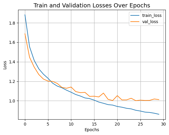
我們剛訓練的 CCT 模型只有 40 萬 個參數,而且在 30 個 epoch 內就達到約 79% 的 top-1 準確度。上面的圖表也顯示沒有過擬合的跡象。這表示我們可以訓練這個網路更久(也許可以稍微增加正規化),並可能獲得更好的效能。這個效能還可以透過其他技巧來進一步提升,像是餘弦退火學習率排程、其他資料擴增技術,例如 AutoAugment、MixUp 或 Cutmix。透過這些修改,作者在 CIFAR-10 資料集上達到 95.1% 的 top-1 準確度。作者還進行了一些實驗,研究卷積區塊、Transformer 層等的數量如何影響 CCT 的最終效能。
作為比較,一個 ViT 模型需要大約 470 萬 個參數和 100 個 epoch 的訓練,才能在 CIFAR-10 資料集上達到 78.22% 的 top-1 準確度。您可以參考 這個筆記本,了解實驗設置。
作者還展示了 Compact Convolutional Transformers 在 NLP 任務上的效能,並報告了具競爭力的結果。