使用監督式一致性訓練
作者: Sayak Paul
建立日期 2021/04/13
上次修改日期 2021/04/19
描述: 使用一致性正規化進行訓練,以提高對抗資料分佈偏移的穩健性。

當資料獨立且同分布 (i.i.d.) 時,深度學習模型在許多影像辨識任務中表現出色。然而,它們可能會因輸入資料中的細微分佈偏移(例如隨機雜訊、對比度變化和模糊)而導致效能下降。因此,自然而然地產生了一個問題,為什麼會這樣?正如 電腦視覺中模型穩健性的傅立葉觀點中所討論的那樣,深度學習模型沒有理由對此類偏移具有穩健性。標準模型訓練程序(例如標準影像分類訓練工作流程)無法讓模型學習超出以訓練資料形式餵給它的內容。
在此範例中,我們將訓練一個影像分類模型,透過執行以下操作,在模型內部強制執行一種一致性的概念:
- 訓練一個標準的影像分類模型。
- 在資料集的雜訊版本上訓練一個相同或更大的模型(使用 RandAugment 擴增)。
- 為此,我們將首先取得先前模型在資料集乾淨影像上的預測。
- 然後,我們將使用這些預測,並訓練第二個模型,使其在相同影像的雜訊變體上匹配這些預測。這與 知識蒸餾 的工作流程相同,但由於學生模型的大小相等或更大,因此此過程也稱為自我訓練。
此整體訓練工作流程的根源在於 FixMatch、用於一致性訓練的無監督資料擴增 和 雜訊學生訓練 等作品。由於此訓練過程鼓勵模型針對乾淨和雜訊影像產生一致的預測,因此它通常被稱為一致性訓練或使用一致性正規化進行訓練。儘管此範例側重於使用一致性訓練來增強模型對常見損壞的穩健性,但此範例也可以作為執行弱監督學習的範本。
此範例需要 TensorFlow 2.4 或更高版本,以及 TensorFlow Hub 和 TensorFlow Models,可以使用以下命令安裝:
!pip install -q tf-models-official tensorflow-addons
導入和設定
from official.vision.image_classification.augment import RandAugment
from tensorflow.keras import layers

import tensorflow as tf
import tensorflow_addons as tfa
import matplotlib.pyplot as plt

tf.random.set_seed(42)
定義超參數
AUTO = tf.data.AUTOTUNE
BATCH_SIZE = 128
EPOCHS = 5

CROP_TO = 72
RESIZE_TO = 96
載入 CIFAR-10 資料集
(x_train, y_train), (x_test, y_test) = tf.keras.datasets.cifar10.load_data()

val_samples = 49500
new_train_x, new_y_train = x_train[: val_samples + 1], y_train[: val_samples + 1]
val_x, val_y = x_train[val_samples:], y_train[val_samples:]
建立 TensorFlow Dataset 物件
# Initialize `RandAugment` object with 2 layers of
# augmentation transforms and strength of 9.
augmenter = RandAugment(num_layers=2, magnitude=9)
為了訓練教師模型,我們將只使用兩種幾何擴增轉換:隨機水平翻轉和隨機裁剪。
def preprocess_train(image, label, noisy=True):
    image = tf.image.random_flip_left_right(image)
    # We first resize the original image to a larger dimension
    # and then we take random crops from it.
    image = tf.image.resize(image, [RESIZE_TO, RESIZE_TO])
    image = tf.image.random_crop(image, [CROP_TO, CROP_TO, 3])
    if noisy:
        image = augmenter.distort(image)
    return image, label


def preprocess_test(image, label):
    image = tf.image.resize(image, [CROP_TO, CROP_TO])
    return image, label


train_ds = tf.data.Dataset.from_tensor_slices((new_train_x, new_y_train))
validation_ds = tf.data.Dataset.from_tensor_slices((val_x, val_y))
test_ds = tf.data.Dataset.from_tensor_slices((x_test, y_test))
我們確保使用相同的種子對 train_clean_ds 和 train_noisy_ds 進行洗牌,以確保它們的順序完全相同。這將在訓練學生模型期間很有幫助。
# This dataset will be used to train the first model.
train_clean_ds = (
    train_ds.shuffle(BATCH_SIZE * 10, seed=42)
    .map(lambda x, y: (preprocess_train(x, y, noisy=False)), num_parallel_calls=AUTO)
    .batch(BATCH_SIZE)
    .prefetch(AUTO)
)

# This prepares the `Dataset` object to use RandAugment.
train_noisy_ds = (
    train_ds.shuffle(BATCH_SIZE * 10, seed=42)
    .map(preprocess_train, num_parallel_calls=AUTO)
    .batch(BATCH_SIZE)
    .prefetch(AUTO)
)

validation_ds = (
    validation_ds.map(preprocess_test, num_parallel_calls=AUTO)
    .batch(BATCH_SIZE)
    .prefetch(AUTO)
)

test_ds = (
    test_ds.map(preprocess_test, num_parallel_calls=AUTO)
    .batch(BATCH_SIZE)
    .prefetch(AUTO)
)

# This dataset will be used to train the second model.
consistency_training_ds = tf.data.Dataset.zip((train_clean_ds, train_noisy_ds))
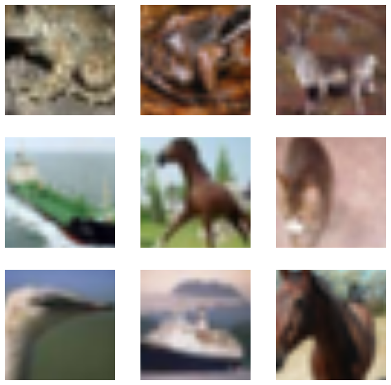
視覺化資料集
sample_images, sample_labels = next(iter(train_clean_ds))
plt.figure(figsize=(10, 10))
for i, image in enumerate(sample_images[:9]):
ax = plt.subplot(3, 3, i + 1)
plt.imshow(image.numpy().astype("int"))
plt.axis("off")
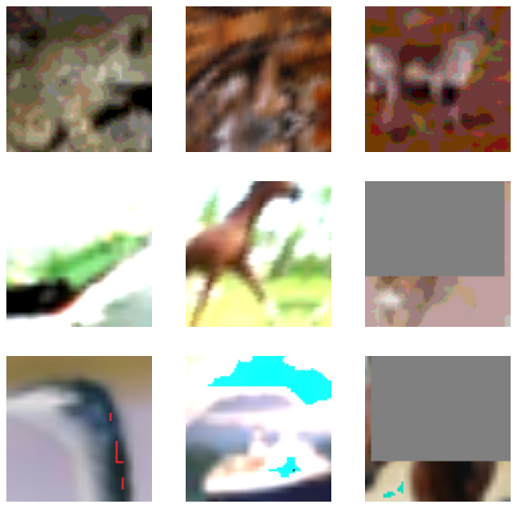
sample_images, sample_labels = next(iter(train_noisy_ds))
plt.figure(figsize=(10, 10))
for i, image in enumerate(sample_images[:9]):
ax = plt.subplot(3, 3, i + 1)
plt.imshow(image.numpy().astype("int"))
plt.axis("off")
定義模型建構公用程式函式
我們現在定義我們的模型建構公用程式。我們的模型基於 ResNet50V2 架構。
def get_training_model(num_classes=10):
    resnet50_v2 = tf.keras.applications.ResNet50V2(
        weights=None, include_top=False, input_shape=(CROP_TO, CROP_TO, 3),
    )
    model = tf.keras.Sequential(
        [
            layers.Input((CROP_TO, CROP_TO, 3)),
            layers.Rescaling(scale=1.0 / 127.5, offset=-1),
            resnet50_v2,
            layers.GlobalAveragePooling2D(),
            layers.Dense(num_classes),
        ]
    )
    return model
為了實現可重複性,我們序列化教師網路的初始隨機權重。
initial_teacher_model = get_training_model()
initial_teacher_model.save_weights("initial_teacher_model.h5")
訓練教師模型
如雜訊學生訓練中所述,如果教師模型使用幾何集成進行訓練,並且當強制學生模型模仿該模型時,它會帶來更好的效能。原始作品使用 隨機深度 和 Dropout 來引入集成部分,但在此範例中,我們將使用 隨機權重平均 (SWA),它也類似於幾何集成。
# Define the callbacks.
reduce_lr = tf.keras.callbacks.ReduceLROnPlateau(patience=3)
early_stopping = tf.keras.callbacks.EarlyStopping(
    patience=10, restore_best_weights=True
)

# Initialize SWA from tf-hub.
SWA = tfa.optimizers.SWA

# Compile and train the teacher model.
teacher_model = get_training_model()
teacher_model.load_weights("initial_teacher_model.h5")
teacher_model.compile(
    # Notice that we are wrapping our optimizer within SWA
    optimizer=SWA(tf.keras.optimizers.Adam()),
    loss=tf.keras.losses.SparseCategoricalCrossentropy(from_logits=True),
    metrics=["accuracy"],
)
history = teacher_model.fit(
    train_clean_ds,
    epochs=EPOCHS,
    validation_data=validation_ds,
    callbacks=[reduce_lr, early_stopping],
)

# Evaluate the teacher model on the test set.
_, acc = teacher_model.evaluate(test_ds, verbose=0)
print(f"Test accuracy: {acc*100}%")
Epoch 1/5
387/387 [==============================] - 73s 78ms/step - loss: 1.7785 - accuracy: 0.3582 - val_loss: 2.0589 - val_accuracy: 0.3920
Epoch 2/5
387/387 [==============================] - 28s 71ms/step - loss: 1.2493 - accuracy: 0.5542 - val_loss: 1.4228 - val_accuracy: 0.5380
Epoch 3/5
387/387 [==============================] - 28s 73ms/step - loss: 1.0294 - accuracy: 0.6350 - val_loss: 1.4422 - val_accuracy: 0.5900
Epoch 4/5
387/387 [==============================] - 28s 73ms/step - loss: 0.8954 - accuracy: 0.6864 - val_loss: 1.2189 - val_accuracy: 0.6520
Epoch 5/5
387/387 [==============================] - 28s 73ms/step - loss: 0.7879 - accuracy: 0.7231 - val_loss: 0.9790 - val_accuracy: 0.6500
Test accuracy: 65.83999991416931%
定義自我訓練公用程式
對於這部分,我們將從 此 Keras 範例中借用 Distiller 類別。
# Majority of the code is taken from:
# https://keras.dev.org.tw/examples/vision/knowledge_distillation/
class SelfTrainer(tf.keras.Model):
    def __init__(self, student, teacher):
        super().__init__()
        self.student = student
        self.teacher = teacher

    def compile(
        self, optimizer, metrics, student_loss_fn, distillation_loss_fn, temperature=3,
    ):
        super().compile(optimizer=optimizer, metrics=metrics)
        self.student_loss_fn = student_loss_fn
        self.distillation_loss_fn = distillation_loss_fn
        self.temperature = temperature

    def train_step(self, data):
        # Since our dataset is a zip of two independent datasets,
        # after initially parsing them, we segregate the
        # respective images and labels next.
        clean_ds, noisy_ds = data
        clean_images, _ = clean_ds
        noisy_images, y = noisy_ds

        # Forward pass of teacher
        teacher_predictions = self.teacher(clean_images, training=False)

        with tf.GradientTape() as tape:
            # Forward pass of student
            student_predictions = self.student(noisy_images, training=True)

            # Compute losses
            student_loss = self.student_loss_fn(y, student_predictions)
            distillation_loss = self.distillation_loss_fn(
                tf.nn.softmax(teacher_predictions / self.temperature, axis=1),
                tf.nn.softmax(student_predictions / self.temperature, axis=1),
            )
            total_loss = (student_loss + distillation_loss) / 2

        # Compute gradients
        trainable_vars = self.student.trainable_variables
        gradients = tape.gradient(total_loss, trainable_vars)

        # Update weights
        self.optimizer.apply_gradients(zip(gradients, trainable_vars))

        # Update the metrics configured in `compile()`
        self.compiled_metrics.update_state(
            y, tf.nn.softmax(student_predictions, axis=1)
        )

        # Return a dict of performance
        results = {m.name: m.result() for m in self.metrics}
        results.update({"total_loss": total_loss})
        return results

    def test_step(self, data):
        # During inference, we only pass a dataset consisting images and labels.
        x, y = data

        # Compute predictions
        y_prediction = self.student(x, training=False)

        # Update the metrics
        self.compiled_metrics.update_state(y, tf.nn.softmax(y_prediction, axis=1))

        # Return a dict of performance
        results = {m.name: m.result() for m in self.metrics}
        return results
此實作中唯一的差異是損失計算的方式。我們不是以不同方式加權蒸餾損失和學生損失,而是根據雜訊學生訓練取它們的平均值。
訓練學生模型
# Define the callbacks.
# We are using a larger decay factor to stabilize the training.
reduce_lr = tf.keras.callbacks.ReduceLROnPlateau(
    patience=3, factor=0.5, monitor="val_accuracy"
)
early_stopping = tf.keras.callbacks.EarlyStopping(
    patience=10, restore_best_weights=True, monitor="val_accuracy"
)

# Compile and train the student model.
self_trainer = SelfTrainer(student=get_training_model(), teacher=teacher_model)
self_trainer.compile(
    # Notice we are *not* using SWA here.
    optimizer="adam",
    metrics=["accuracy"],
    student_loss_fn=tf.keras.losses.SparseCategoricalCrossentropy(from_logits=True),
    distillation_loss_fn=tf.keras.losses.KLDivergence(),
    temperature=10,
)
history = self_trainer.fit(
    consistency_training_ds,
    epochs=EPOCHS,
    validation_data=validation_ds,
    callbacks=[reduce_lr, early_stopping],
)

# Evaluate the student model.
acc = self_trainer.evaluate(test_ds, verbose=0)
print(f"Test accuracy from student model: {acc*100}%")
Epoch 1/5
387/387 [==============================] - 39s 84ms/step - accuracy: 0.2112 - total_loss: 1.0629 - val_accuracy: 0.4180
Epoch 2/5
387/387 [==============================] - 32s 82ms/step - accuracy: 0.3341 - total_loss: 0.9554 - val_accuracy: 0.3900
Epoch 3/5
387/387 [==============================] - 31s 81ms/step - accuracy: 0.3873 - total_loss: 0.8852 - val_accuracy: 0.4580
Epoch 4/5
387/387 [==============================] - 31s 81ms/step - accuracy: 0.4294 - total_loss: 0.8423 - val_accuracy: 0.5660
Epoch 5/5
387/387 [==============================] - 31s 81ms/step - accuracy: 0.4547 - total_loss: 0.8093 - val_accuracy: 0.5880
Test accuracy from student model: 58.490002155303955%
評估模型的穩健性
評估視覺模型穩健性的標準基準是在損壞的資料集(如 ImageNet-C 和 CIFAR-10-C)上記錄它們的效能,這兩個資料集都在 針對常見損壞和擾動評估神經網路穩健性 中提出。對於此範例,我們將使用 CIFAR-10-C 資料集,該資料集在 5 個不同的嚴重程度層級上有 19 種不同的損壞。為了評估模型在此資料集上的穩健性,我們將執行以下操作:
- 在最高嚴重程度層級上執行預訓練模型,並取得 top-1 準確度。
- 計算平均 top-1 準確度。
為了這個範例的目的,我們不會逐步執行這些步驟。這也是為什麼我們只訓練模型 5 個 epoch 的原因。您可以查看這個儲存庫,其中展示了完整規模的訓練實驗,以及上述的評估。下圖呈現了該評估的執行摘要。

平均 Top-1 結果代表 CIFAR-10-C 資料集,而 測試 Top-1 結果代表 CIFAR-10 測試集。很明顯地,一致性訓練不僅在增強模型穩健性方面具有優勢,在提高標準測試效能方面也具有優勢。