去噪擴散機率模型
作者: A_K_Nain
建立日期 2022/11/30
上次修改日期 2022/12/07
描述: 使用去噪擴散機率模型生成花朵圖像。

簡介
生成式建模在過去五年中經歷了巨大的增長。諸如 VAE、GAN 和基於流的模型等模型在生成高質量內容(尤其是圖像)方面證明了巨大的成功。擴散模型是一種新型的生成模型,已被證明比以前的方法更好。
擴散模型受到非平衡熱力學的啟發,它們學習通過去噪來生成。通過去噪學習包括兩個過程,每個過程都是一個馬可夫鏈。這些是
-
前向過程:在前向過程中,我們在時間序列
(t1, t2, ..., tn )中緩慢地將隨機噪聲添加到資料中。目前時間步的樣本是從高斯分布中提取的,其中分布的平均值以先前時間步的樣本為條件,且分布的變異數遵循固定的時程。在前向過程結束時,樣本最終會呈現純噪聲分布。 -
反向過程:在反向過程中,我們嘗試在每個時間步撤銷添加的噪聲。我們從純噪聲分布(前向過程的最後一步)開始,嘗試在向後方向
(tn, tn-1, ..., t1)對樣本進行去噪。
在此程式碼範例中,我們實作了 去噪擴散機率模型論文,簡稱 DDPM。這是第一篇展示使用擴散模型生成高質量圖像的論文。作者證明了擴散模型的某些參數化顯示了在訓練期間對多個噪聲級別進行去噪分數匹配,以及在採樣期間使用退火朗之萬動力學(產生最佳質量結果)的等效性。
這篇論文複製了擴散過程中涉及的兩個馬可夫鏈(前向過程和反向過程),但用於圖像。前向過程是固定的,並根據論文中以 beta 表示的固定變異數時程,逐漸向圖像添加高斯噪聲。以下是圖像的擴散過程:(圖像 -> 噪聲::噪聲 -> 圖像)
該論文描述了兩種演算法,一種用於訓練模型,另一種用於從訓練好的模型中採樣。訓練是通過優化負對數似然的通常變分界限來執行的。目標函數進一步簡化,並且網路被視為噪聲預測網路。一旦優化,我們就可以從網路中採樣,以從噪聲樣本生成新的圖像。以下是論文中提出的兩種演算法的概述

注意: DDPM 只是實作擴散模型的一種方法。此外,DDPM 中的採樣演算法複製了完整的馬可夫鏈。因此,與 GAN 等其他生成模型相比,它在生成新樣本時速度較慢。為了解決這個問題,已經做了很多研究工作。一個這樣的例子是去噪擴散隱式模型,簡稱 DDIM,其中作者用非馬可夫過程取代了馬可夫鏈,以加快採樣速度。您可以在這裡找到 DDIM 的程式碼範例
實作 DDPM 模型很簡單。我們定義一個模型,該模型接收兩個輸入:圖像和隨機採樣的時間步。在每個訓練步驟中,我們執行以下操作來訓練我們的模型
- 採樣要添加到輸入的隨機噪聲。
- 應用前向過程以使用採樣的噪聲擴散輸入。
- 您的模型將這些嘈雜的樣本作為輸入,並輸出每個時間步的噪聲預測。
- 給定真實噪聲和預測噪聲,我們計算損失值
- 然後,我們計算梯度並更新模型權重。
鑑於我們的模型知道如何在給定時間步對嘈雜的樣本進行去噪,我們可以利用這個想法來生成新樣本,從純噪聲分布開始。
設定
import math
import numpy as np
import matplotlib.pyplot as plt

# Requires TensorFlow >=2.11 for the GroupNormalization layer.
import tensorflow as tf
from tensorflow import keras
from tensorflow.keras import layers
import tensorflow_datasets as tfds
超參數
batch_size = 32
num_epochs = 1  # Just for the sake of demonstration
total_timesteps = 1000
norm_groups = 8  # Number of groups used in GroupNormalization layer
learning_rate = 2e-4

img_size = 64
img_channels = 3
clip_min = -1.0
clip_max = 1.0

first_conv_channels = 64
channel_multiplier = [1, 2, 4, 8]
widths = [first_conv_channels * mult for mult in channel_multiplier]
has_attention = [False, False, True, True]
num_res_blocks = 2  # Number of residual blocks

dataset_name = "oxford_flowers102"
splits = ["train"]
資料集
我們使用 牛津花卉 102 資料集生成花卉圖像。在預處理方面,我們使用中心裁剪將圖像調整為所需的圖像大小,並將像素值重新縮放到 [-1.0, 1.0] 的範圍內。這與 DDPM 論文的作者應用的像素值範圍一致。為了擴增訓練資料,我們隨機左右翻轉圖像。
# Load the dataset
(ds,) = tfds.load(dataset_name, split=splits, with_info=False, shuffle_files=True)


def augment(img):
    """Flips an image left/right randomly."""
    return tf.image.random_flip_left_right(img)


def resize_and_rescale(img, size):
    """Resize the image to the desired size first and then
    rescale the pixel values in the range [-1.0, 1.0].

    Args:
        img: Image tensor
        size: Desired image size for resizing
    Returns:
        Resized and rescaled image tensor
    """

    height = tf.shape(img)[0]
    width = tf.shape(img)[1]
    crop_size = tf.minimum(height, width)

    img = tf.image.crop_to_bounding_box(
        img,
        (height - crop_size) // 2,
        (width - crop_size) // 2,
        crop_size,
        crop_size,
    )

    # Resize
    img = tf.cast(img, dtype=tf.float32)
    img = tf.image.resize(img, size=size, antialias=True)

    # Rescale the pixel values
    img = img / 127.5 - 1.0
    img = tf.clip_by_value(img, clip_min, clip_max)
    return img


def train_preprocessing(x):
    img = x["image"]
    img = resize_and_rescale(img, size=(img_size, img_size))
    img = augment(img)
    return img


train_ds = (
    ds.map(train_preprocessing, num_parallel_calls=tf.data.AUTOTUNE)
    .batch(batch_size, drop_remainder=True)
    .shuffle(batch_size * 2)
    .prefetch(tf.data.AUTOTUNE)
)
高斯擴散實用程式
我們將前向過程和反向過程定義為單獨的實用程式。此實用程式中的大部分程式碼都借用了原始實作,並進行了一些細微的修改。
class GaussianDiffusion:
    """Gaussian diffusion utility.

    Args:
        beta_start: Start value of the scheduled variance
        beta_end: End value of the scheduled variance
        timesteps: Number of time steps in the forward process
    """

    def __init__(
        self,
        beta_start=1e-4,
        beta_end=0.02,
        timesteps=1000,
        clip_min=-1.0,
        clip_max=1.0,
    ):
        self.beta_start = beta_start
        self.beta_end = beta_end
        self.timesteps = timesteps
        self.clip_min = clip_min
        self.clip_max = clip_max

        # Define the linear variance schedule
        self.betas = betas = np.linspace(
            beta_start,
            beta_end,
            timesteps,
            dtype=np.float64,  # Using float64 for better precision
        )
        self.num_timesteps = int(timesteps)

        alphas = 1.0 - betas
        alphas_cumprod = np.cumprod(alphas, axis=0)
        alphas_cumprod_prev = np.append(1.0, alphas_cumprod[:-1])

        self.betas = tf.constant(betas, dtype=tf.float32)
        self.alphas_cumprod = tf.constant(alphas_cumprod, dtype=tf.float32)
        self.alphas_cumprod_prev = tf.constant(alphas_cumprod_prev, dtype=tf.float32)

        # Calculations for diffusion q(x_t | x_{t-1}) and others
        self.sqrt_alphas_cumprod = tf.constant(
            np.sqrt(alphas_cumprod), dtype=tf.float32
        )

        self.sqrt_one_minus_alphas_cumprod = tf.constant(
            np.sqrt(1.0 - alphas_cumprod), dtype=tf.float32
        )

        self.log_one_minus_alphas_cumprod = tf.constant(
            np.log(1.0 - alphas_cumprod), dtype=tf.float32
        )

        self.sqrt_recip_alphas_cumprod = tf.constant(
            np.sqrt(1.0 / alphas_cumprod), dtype=tf.float32
        )
        self.sqrt_recipm1_alphas_cumprod = tf.constant(
            np.sqrt(1.0 / alphas_cumprod - 1), dtype=tf.float32
        )

        # Calculations for posterior q(x_{t-1} | x_t, x_0)
        posterior_variance = (
            betas * (1.0 - alphas_cumprod_prev) / (1.0 - alphas_cumprod)
        )
        self.posterior_variance = tf.constant(posterior_variance, dtype=tf.float32)

        # Log calculation clipped because the posterior variance is 0 at the beginning
        # of the diffusion chain
        self.posterior_log_variance_clipped = tf.constant(
            np.log(np.maximum(posterior_variance, 1e-20)), dtype=tf.float32
        )

        self.posterior_mean_coef1 = tf.constant(
            betas * np.sqrt(alphas_cumprod_prev) / (1.0 - alphas_cumprod),
            dtype=tf.float32,
        )

        self.posterior_mean_coef2 = tf.constant(
            (1.0 - alphas_cumprod_prev) * np.sqrt(alphas) / (1.0 - alphas_cumprod),
            dtype=tf.float32,
        )

    def _extract(self, a, t, x_shape):
        """Extract some coefficients at specified timesteps,
        then reshape to [batch_size, 1, 1, 1, 1, ...] for broadcasting purposes.

        Args:
            a: Tensor to extract from
            t: Timestep for which the coefficients are to be extracted
            x_shape: Shape of the current batched samples
        """
        batch_size = x_shape[0]
        out = tf.gather(a, t)
        return tf.reshape(out, [batch_size, 1, 1, 1])

    def q_mean_variance(self, x_start, t):
        """Extracts the mean, and the variance at current timestep.

        Args:
            x_start: Initial sample (before the first diffusion step)
            t: Current timestep
        """
        x_start_shape = tf.shape(x_start)
        mean = self._extract(self.sqrt_alphas_cumprod, t, x_start_shape) * x_start
        variance = self._extract(1.0 - self.alphas_cumprod, t, x_start_shape)
        log_variance = self._extract(
            self.log_one_minus_alphas_cumprod, t, x_start_shape
        )
        return mean, variance, log_variance

    def q_sample(self, x_start, t, noise):
        """Diffuse the data.

        Args:
            x_start: Initial sample (before the first diffusion step)
            t: Current timestep
            noise: Gaussian noise to be added at the current timestep
        Returns:
            Diffused samples at timestep `t`
        """
        x_start_shape = tf.shape(x_start)
        return (
            self._extract(self.sqrt_alphas_cumprod, t, tf.shape(x_start)) * x_start
            + self._extract(self.sqrt_one_minus_alphas_cumprod, t, x_start_shape)
            * noise
        )

    def predict_start_from_noise(self, x_t, t, noise):
        x_t_shape = tf.shape(x_t)
        return (
            self._extract(self.sqrt_recip_alphas_cumprod, t, x_t_shape) * x_t
            - self._extract(self.sqrt_recipm1_alphas_cumprod, t, x_t_shape) * noise
        )

    def q_posterior(self, x_start, x_t, t):
        """Compute the mean and variance of the diffusion
        posterior q(x_{t-1} | x_t, x_0).

        Args:
            x_start: Stating point(sample) for the posterior computation
            x_t: Sample at timestep `t`
            t: Current timestep
        Returns:
            Posterior mean and variance at current timestep
        """

        x_t_shape = tf.shape(x_t)
        posterior_mean = (
            self._extract(self.posterior_mean_coef1, t, x_t_shape) * x_start
            + self._extract(self.posterior_mean_coef2, t, x_t_shape) * x_t
        )
        posterior_variance = self._extract(self.posterior_variance, t, x_t_shape)
        posterior_log_variance_clipped = self._extract(
            self.posterior_log_variance_clipped, t, x_t_shape
        )
        return posterior_mean, posterior_variance, posterior_log_variance_clipped

    def p_mean_variance(self, pred_noise, x, t, clip_denoised=True):
        x_recon = self.predict_start_from_noise(x, t=t, noise=pred_noise)
        if clip_denoised:
            x_recon = tf.clip_by_value(x_recon, self.clip_min, self.clip_max)

        model_mean, posterior_variance, posterior_log_variance = self.q_posterior(
            x_start=x_recon, x_t=x, t=t
        )
        return model_mean, posterior_variance, posterior_log_variance

    def p_sample(self, pred_noise, x, t, clip_denoised=True):
        """Sample from the diffusion model.

        Args:
            pred_noise: Noise predicted by the diffusion model
            x: Samples at a given timestep for which the noise was predicted
            t: Current timestep
            clip_denoised (bool): Whether to clip the predicted noise
                within the specified range or not.
        """
        model_mean, _, model_log_variance = self.p_mean_variance(
            pred_noise, x=x, t=t, clip_denoised=clip_denoised
        )
        noise = tf.random.normal(shape=x.shape, dtype=x.dtype)
        # No noise when t == 0
        nonzero_mask = tf.reshape(
            1 - tf.cast(tf.equal(t, 0), tf.float32), [tf.shape(x)[0], 1, 1, 1]
        )
        return model_mean + nonzero_mask * tf.exp(0.5 * model_log_variance) * noise
網路架構
U-Net 最初是為語義分割開發的,是一種廣泛用於實作擴散模型的架構,但進行了一些細微的修改
- 該網路接受兩個輸入:圖像和時間步
- 一旦我們達到特定的解析度(論文中為 16x16),卷積區塊之間的自我注意
- 群組正規化而不是權重正規化
我們實作了原始論文中使用的大部分內容。我們在整個網路中使用 swish 激活函數。我們使用變異數縮放核心初始化器。
這裡唯一的區別是 GroupNormalization 層使用的群組數。對於花卉資料集,我們發現值為 groups=8 的結果比預設值 groups=32 更好。Dropout 是可選的,應在過度擬合的機會很高的地方使用。在論文中,作者僅在 CIFAR10 上進行訓練時使用了 dropout。
# Kernel initializer to use
def kernel_init(scale):
    scale = max(scale, 1e-10)
    return keras.initializers.VarianceScaling(
        scale, mode="fan_avg", distribution="uniform"
    )


class AttentionBlock(layers.Layer):
    """Applies self-attention.

    Args:
        units: Number of units in the dense layers
        groups: Number of groups to be used for GroupNormalization layer
    """

    def __init__(self, units, groups=8, **kwargs):
        self.units = units
        self.groups = groups
        super().__init__(**kwargs)

        self.norm = layers.GroupNormalization(groups=groups)
        self.query = layers.Dense(units, kernel_initializer=kernel_init(1.0))
        self.key = layers.Dense(units, kernel_initializer=kernel_init(1.0))
        self.value = layers.Dense(units, kernel_initializer=kernel_init(1.0))
        self.proj = layers.Dense(units, kernel_initializer=kernel_init(0.0))

    def call(self, inputs):
        batch_size = tf.shape(inputs)[0]
        height = tf.shape(inputs)[1]
        width = tf.shape(inputs)[2]
        scale = tf.cast(self.units, tf.float32) ** (-0.5)

        inputs = self.norm(inputs)
        q = self.query(inputs)
        k = self.key(inputs)
        v = self.value(inputs)

        attn_score = tf.einsum("bhwc, bHWc->bhwHW", q, k) * scale
        attn_score = tf.reshape(attn_score, [batch_size, height, width, height * width])

        attn_score = tf.nn.softmax(attn_score, -1)
        attn_score = tf.reshape(attn_score, [batch_size, height, width, height, width])

        proj = tf.einsum("bhwHW,bHWc->bhwc", attn_score, v)
        proj = self.proj(proj)
        return inputs + proj


class TimeEmbedding(layers.Layer):
    def __init__(self, dim, **kwargs):
        super().__init__(**kwargs)
        self.dim = dim
        self.half_dim = dim // 2
        self.emb = math.log(10000) / (self.half_dim - 1)
        self.emb = tf.exp(tf.range(self.half_dim, dtype=tf.float32) * -self.emb)

    def call(self, inputs):
        inputs = tf.cast(inputs, dtype=tf.float32)
        emb = inputs[:, None] * self.emb[None, :]
        emb = tf.concat([tf.sin(emb), tf.cos(emb)], axis=-1)
        return emb


def ResidualBlock(width, groups=8, activation_fn=keras.activations.swish):
    def apply(inputs):
        x, t = inputs
        input_width = x.shape[3]

        if input_width == width:
            residual = x
        else:
            residual = layers.Conv2D(
                width, kernel_size=1, kernel_initializer=kernel_init(1.0)
            )(x)

        temb = activation_fn(t)
        temb = layers.Dense(width, kernel_initializer=kernel_init(1.0))(temb)[
            :, None, None, :
        ]

        x = layers.GroupNormalization(groups=groups)(x)
        x = activation_fn(x)
        x = layers.Conv2D(
            width, kernel_size=3, padding="same", kernel_initializer=kernel_init(1.0)
        )(x)

        x = layers.Add()([x, temb])
        x = layers.GroupNormalization(groups=groups)(x)
        x = activation_fn(x)

        x = layers.Conv2D(
            width, kernel_size=3, padding="same", kernel_initializer=kernel_init(0.0)
        )(x)
        x = layers.Add()([x, residual])
        return x

    return apply


def DownSample(width):
    def apply(x):
        x = layers.Conv2D(
            width,
            kernel_size=3,
            strides=2,
            padding="same",
            kernel_initializer=kernel_init(1.0),
        )(x)
        return x

    return apply


def UpSample(width, interpolation="nearest"):
    def apply(x):
        x = layers.UpSampling2D(size=2, interpolation=interpolation)(x)
        x = layers.Conv2D(
            width, kernel_size=3, padding="same", kernel_initializer=kernel_init(1.0)
        )(x)
        return x

    return apply


def TimeMLP(units, activation_fn=keras.activations.swish):
    def apply(inputs):
        temb = layers.Dense(
            units, activation=activation_fn, kernel_initializer=kernel_init(1.0)
        )(inputs)
        temb = layers.Dense(units, kernel_initializer=kernel_init(1.0))(temb)
        return temb

    return apply


def build_model(
    img_size,
    img_channels,
    widths,
    has_attention,
    num_res_blocks=2,
    norm_groups=8,
    interpolation="nearest",
    activation_fn=keras.activations.swish,
):
    image_input = layers.Input(
        shape=(img_size, img_size, img_channels), name="image_input"
    )
    time_input = keras.Input(shape=(), dtype=tf.int64, name="time_input")

    x = layers.Conv2D(
        first_conv_channels,
        kernel_size=(3, 3),
        padding="same",
        kernel_initializer=kernel_init(1.0),
    )(image_input)

    temb = TimeEmbedding(dim=first_conv_channels * 4)(time_input)
    temb = TimeMLP(units=first_conv_channels * 4, activation_fn=activation_fn)(temb)

    skips = [x]

    # DownBlock
    for i in range(len(widths)):
        for _ in range(num_res_blocks):
            x = ResidualBlock(
                widths[i], groups=norm_groups, activation_fn=activation_fn
            )([x, temb])
            if has_attention[i]:
                x = AttentionBlock(widths[i], groups=norm_groups)(x)
            skips.append(x)

        if widths[i] != widths[-1]:
            x = DownSample(widths[i])(x)
            skips.append(x)

    # MiddleBlock
    x = ResidualBlock(widths[-1], groups=norm_groups, activation_fn=activation_fn)(
        [x, temb]
    )
    x = AttentionBlock(widths[-1], groups=norm_groups)(x)
    x = ResidualBlock(widths[-1], groups=norm_groups, activation_fn=activation_fn)(
        [x, temb]
    )

    # UpBlock
    for i in reversed(range(len(widths))):
        for _ in range(num_res_blocks + 1):
            x = layers.Concatenate(axis=-1)([x, skips.pop()])
            x = ResidualBlock(
                widths[i], groups=norm_groups, activation_fn=activation_fn
            )([x, temb])
            if has_attention[i]:
                x = AttentionBlock(widths[i], groups=norm_groups)(x)

        if i != 0:
            x = UpSample(widths[i], interpolation=interpolation)(x)

    # End block
    x = layers.GroupNormalization(groups=norm_groups)(x)
    x = activation_fn(x)
    x = layers.Conv2D(3, (3, 3), padding="same", kernel_initializer=kernel_init(0.0))(x)
    return keras.Model([image_input, time_input], x, name="unet")
訓練
我們遵循與論文中描述的相同的設定來訓練擴散模型。我們使用學習率為 2e-4 的 Adam 優化器。我們對模型參數使用 EMA,衰減因子為 0.999。我們將模型視為噪聲預測網路,即在每個訓練步驟中,我們將一批圖像和相應的時間步輸入到 UNet,網路輸出噪聲作為預測。
唯一的區別是,我們沒有使用 Kernel Inception Distance (KID) 或 Frechet Inception Distance (FID) 來評估訓練期間產生的樣本的品質。這是因為這兩個指標的計算量都很大,為了簡潔起見,被省略了。
**注意:** 我們正在使用均方誤差作為損失函數,這與論文一致,並且在理論上是有意義的。但是,在實務上,使用平均絕對誤差或 Huber 損失作為損失函數也很常見。
class DiffusionModel(keras.Model):
    def __init__(self, network, ema_network, timesteps, gdf_util, ema=0.999):
        super().__init__()
        self.network = network
        self.ema_network = ema_network
        self.timesteps = timesteps
        self.gdf_util = gdf_util
        self.ema = ema

    def train_step(self, images):
        # 1. Get the batch size
        batch_size = tf.shape(images)[0]

        # 2. Sample timesteps uniformly
        t = tf.random.uniform(
            minval=0, maxval=self.timesteps, shape=(batch_size,), dtype=tf.int64
        )

        with tf.GradientTape() as tape:
            # 3. Sample random noise to be added to the images in the batch
            noise = tf.random.normal(shape=tf.shape(images), dtype=images.dtype)

            # 4. Diffuse the images with noise
            images_t = self.gdf_util.q_sample(images, t, noise)

            # 5. Pass the diffused images and time steps to the network
            pred_noise = self.network([images_t, t], training=True)

            # 6. Calculate the loss
            loss = self.loss(noise, pred_noise)

        # 7. Get the gradients
        gradients = tape.gradient(loss, self.network.trainable_weights)

        # 8. Update the weights of the network
        self.optimizer.apply_gradients(zip(gradients, self.network.trainable_weights))

        # 9. Updates the weight values for the network with EMA weights
        for weight, ema_weight in zip(self.network.weights, self.ema_network.weights):
            ema_weight.assign(self.ema * ema_weight + (1 - self.ema) * weight)

        # 10. Return loss values
        return {"loss": loss}

    def generate_images(self, num_images=16):
        # 1. Randomly sample noise (starting point for reverse process)
        samples = tf.random.normal(
            shape=(num_images, img_size, img_size, img_channels), dtype=tf.float32
        )
        # 2. Sample from the model iteratively
        for t in reversed(range(0, self.timesteps)):
            tt = tf.cast(tf.fill(num_images, t), dtype=tf.int64)
            pred_noise = self.ema_network.predict(
                [samples, tt], verbose=0, batch_size=num_images
            )
            samples = self.gdf_util.p_sample(
                pred_noise, samples, tt, clip_denoised=True
            )
        # 3. Return generated samples
        return samples

    def plot_images(
        self, epoch=None, logs=None, num_rows=2, num_cols=8, figsize=(12, 5)
    ):
        """Utility to plot images using the diffusion model during training."""
        generated_samples = self.generate_images(num_images=num_rows * num_cols)
        generated_samples = (
            tf.clip_by_value(generated_samples * 127.5 + 127.5, 0.0, 255.0)
            .numpy()
            .astype(np.uint8)
        )

        _, ax = plt.subplots(num_rows, num_cols, figsize=figsize)
        for i, image in enumerate(generated_samples):
            if num_rows == 1:
                ax[i].imshow(image)
                ax[i].axis("off")
            else:
                ax[i // num_cols, i % num_cols].imshow(image)
                ax[i // num_cols, i % num_cols].axis("off")

        plt.tight_layout()
        plt.show()


# Build the unet model
network = build_model(
    img_size=img_size,
    img_channels=img_channels,
    widths=widths,
    has_attention=has_attention,
    num_res_blocks=num_res_blocks,
    norm_groups=norm_groups,
    activation_fn=keras.activations.swish,
)
ema_network = build_model(
    img_size=img_size,
    img_channels=img_channels,
    widths=widths,
    has_attention=has_attention,
    num_res_blocks=num_res_blocks,
    norm_groups=norm_groups,
    activation_fn=keras.activations.swish,
)
ema_network.set_weights(network.get_weights())  # Initially the weights are the same

# Get an instance of the Gaussian Diffusion utilities
gdf_util = GaussianDiffusion(timesteps=total_timesteps)

# Get the model
model = DiffusionModel(
    network=network,
    ema_network=ema_network,
    gdf_util=gdf_util,
    timesteps=total_timesteps,
)

# Compile the model
model.compile(
    loss=keras.losses.MeanSquaredError(),
    optimizer=keras.optimizers.Adam(learning_rate=learning_rate),
)

# Train the model
model.fit(
    train_ds,
    epochs=num_epochs,
    batch_size=batch_size,
    callbacks=[keras.callbacks.LambdaCallback(on_epoch_end=model.plot_images)],
)
31/31 [==============================] - ETA: 0s - loss: 0.7746
31/31 [==============================] - 194s 4s/step - loss: 0.7668

<keras.callbacks.History at 0x7fc9e86ce610>
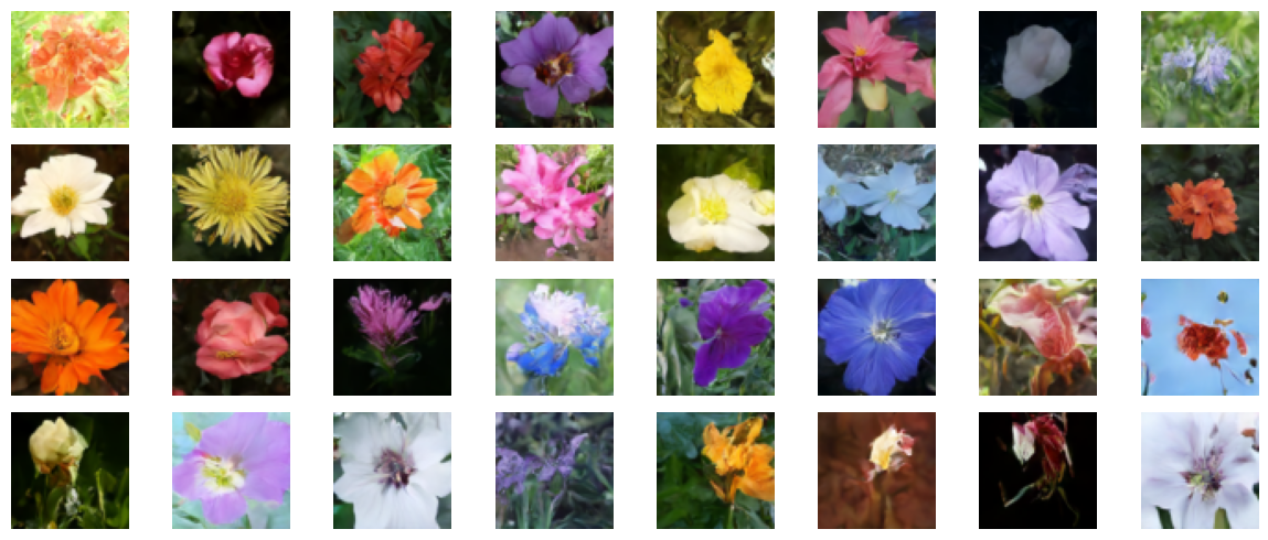
結果
我們在 V100 GPU 上訓練此模型 800 個 epoch,每個 epoch 幾乎需要 8 秒才能完成。我們在這裡載入這些權重,並從純噪聲開始生成一些樣本。
!curl -LO https://github.com/AakashKumarNain/ddpms/releases/download/v3.0.0/checkpoints.zip
!unzip -qq checkpoints.zip
# Load the model weights
model.ema_network.load_weights("checkpoints/diffusion_model_checkpoint")

# Generate and plot some samples
model.plot_images(num_rows=4, num_cols=8)
  % Total    % Received % Xferd  Average Speed   Time    Time     Time  Current
                                 Dload  Upload   Total   Spent    Left  Speed
  0     0    0     0    0     0      0      0 --:--:-- --:--:-- --:--:--     0
100  222M  100  222M    0     0  16.0M      0  0:00:13  0:00:13 --:--:-- 14.7M
結論
我們成功地實作並訓練了擴散模型,其方式與 DDPM 論文的作者實作的方式完全相同。您可以在這裡找到原始實作。
您可以嘗試一些方法來改進模型
-
增加每個區塊的寬度。較大的模型可以在較少的 epoch 中學習去噪,但您可能必須注意過度擬合。
-
我們實作了用於變異數時程的線性時程。您可以實作其他方案,如餘弦時程,並比較效能。