使用 node2vec 進行圖形表示學習
作者: Khalid Salama
建立日期 2021/05/15
上次修改日期 2021/05/15
描述: 實作 node2vec 模型,從 MovieLens 資料集產生電影的嵌入。

簡介
從結構化為圖形的物件中學習有用的表示法,對於各種機器學習 (ML) 應用程式非常有用,例如社群和通訊網路分析、生物醫學研究和推薦系統。圖形表示學習旨在學習圖形節點的嵌入,這些嵌入可用於各種 ML 任務,例如節點標籤預測 (例如,根據文章的引用對文章進行分類) 和連結預測 (例如,向社群網路中的使用者推薦興趣群組)。
node2vec 是一種簡單、可擴展且有效的方法,透過最佳化保留鄰域的目標,學習圖形中節點的低維嵌入。目標是學習相鄰節點的相似嵌入,與圖形結構相關。
如果您的資料項目結構化為圖形 (其中項目表示為節點,項目之間的關係表示為邊緣),則 node2vec 的運作方式如下:
- 使用(有偏差的)隨機遊走產生項目序列。
- 從這些序列建立正負訓練範例。
- 訓練 word2vec 模型 (skip-gram) 來學習項目的嵌入。
在本範例中,我們將在 Movielens 資料集的小型版本上示範 node2vec 技術,以學習電影嵌入。這種資料集可以表示為圖形,方法是將電影視為節點,並在使用者評分相似的電影之間建立邊緣。學習到的電影嵌入可以用於電影推薦或電影類型預測等任務。
此範例需要 networkx 套件,可以使用下列指令安裝:
pip install networkx
設定
import os
from collections import defaultdict
import math
import networkx as nx
import random
from tqdm import tqdm
from zipfile import ZipFile
from urllib.request import urlretrieve
import numpy as np
import pandas as pd
import tensorflow as tf
from tensorflow import keras
from tensorflow.keras import layers
import matplotlib.pyplot as plt
下載 MovieLens 資料集並準備資料
MovieLens 資料集的小型版本包含約 10 萬個來自 610 位使用者對 9,742 部電影的評分。
首先,我們先下載資料集。下載的資料夾將包含三個資料檔案:users.csv、movies.csv 和 ratings.csv。在本範例中,我們只需要 movies.dat 和 ratings.dat 資料檔案。
urlretrieve(
    "http://files.grouplens.org/datasets/movielens/ml-latest-small.zip", "movielens.zip"
)
ZipFile("movielens.zip", "r").extractall()
然後,我們將資料載入 Pandas DataFrame 並執行一些基本的前處理。
# Load movies to a DataFrame.
movies = pd.read_csv("ml-latest-small/movies.csv")
# Create a `movieId` string.
movies["movieId"] = movies["movieId"].apply(lambda x: f"movie_{x}")

# Load ratings to a DataFrame.
ratings = pd.read_csv("ml-latest-small/ratings.csv")
# Convert the `ratings` to floating point
ratings["rating"] = ratings["rating"].apply(lambda x: float(x))
# Create the `movie_id` string.
ratings["movieId"] = ratings["movieId"].apply(lambda x: f"movie_{x}")

print("Movies data shape:", movies.shape)
print("Ratings data shape:", ratings.shape)
Movies data shape: (9742, 3)
Ratings data shape: (100836, 4)
讓我們檢查 ratings DataFrame 的範例。
ratings.head()
| userId | movieId | rating | timestamp | |
|---|---|---|---|---|
| 0 | 1 | movie_1 | 4.0 | 964982703 |
| 1 | 1 | movie_3 | 4.0 | 964981247 |
| 2 | 1 | movie_6 | 4.0 | 964982224 |
| 3 | 1 | movie_47 | 5.0 | 964983815 |
| 4 | 1 | movie_50 | 5.0 | 964982931 |
接下來,讓我們檢查 movies DataFrame 的範例。
movies.head()
| movieId | title | genres | |
|---|---|---|---|
| 0 | movie_1 | 玩具總動員 (1995) | 冒險|動畫|兒童|喜劇|奇幻 |
| 1 | movie_2 | 野蠻遊戲 (1995) | 冒險|兒童|奇幻 |
| 2 | movie_3 | 古怪老頭 (1995) | 喜劇|愛情 |
| 3 | movie_4 | 等待夢醒時分 (1995) | 喜劇|劇情|愛情 |
| 4 | movie_5 | 新岳父大人 (1995) | 喜劇 |
實作 movies DataFrame 的兩個實用函式。
def get_movie_title_by_id(movieId):
    return list(movies[movies.movieId == movieId].title)[0]


def get_movie_id_by_title(title):
    return list(movies[movies.title == title].movieId)[0]
建構電影圖形
如果兩部電影由同一使用者評分 >= min_rating,我們會在圖形中的兩個電影節點之間建立邊緣。邊緣的權重將基於兩部電影之間的 點向互資訊,其計算方式如下:log(xy) - log(x) - log(y) + log(D),其中
xy是有多少使用者對電影x和電影y的評分都 >=min_rating。x是有多少使用者對電影x的評分 >=min_rating。y是有多少使用者對電影y的評分 >=min_rating。D是評分 >=min_rating的電影總數。
步驟 1:建立電影之間的加權邊緣。
min_rating = 5
pair_frequency = defaultdict(int)
item_frequency = defaultdict(int)

# Filter instances where rating is greater than or equal to min_rating.
rated_movies = ratings[ratings.rating >= min_rating]
# Group instances by user.
movies_grouped_by_users = list(rated_movies.groupby("userId"))
for group in tqdm(
    movies_grouped_by_users,
    position=0,
    leave=True,
    desc="Compute movie rating frequencies",
):
    # Get a list of movies rated by the user.
    current_movies = list(group[1]["movieId"])

    for i in range(len(current_movies)):
        item_frequency[current_movies[i]] += 1
        for j in range(i + 1, len(current_movies)):
            x = min(current_movies[i], current_movies[j])
            y = max(current_movies[i], current_movies[j])
            pair_frequency[(x, y)] += 1
Compute movie rating frequencies: 100%|███████████████████████████████████████████████████████████████████████████| 573/573 [00:00<00:00, 1049.83it/s]
步驟 2:使用節點和邊緣建立圖形
為了減少節點之間的邊緣數量,只有在邊緣的權重高於 min_weight 時,我們才會在電影之間新增邊緣。
min_weight = 10
D = math.log(sum(item_frequency.values()))

# Create the movies undirected graph.
movies_graph = nx.Graph()
# Add weighted edges between movies.
# This automatically adds the movie nodes to the graph.
for pair in tqdm(
    pair_frequency, position=0, leave=True, desc="Creating the movie graph"
):
    x, y = pair
    xy_frequency = pair_frequency[pair]
    x_frequency = item_frequency[x]
    y_frequency = item_frequency[y]
    pmi = math.log(xy_frequency) - math.log(x_frequency) - math.log(y_frequency) + D
    weight = pmi * xy_frequency
    # Only include edges with weight >= min_weight.
    if weight >= min_weight:
        movies_graph.add_edge(x, y, weight=weight)
Creating the movie graph: 100%|███████████████████████████████████████████████████████████████████████████| 298586/298586 [00:00<00:00, 552893.62it/s]
讓我們顯示圖形中的節點和邊緣總數。請注意,節點數量少於電影總數,因為只會新增與其他電影有邊緣的電影。
print("Total number of graph nodes:", movies_graph.number_of_nodes())
print("Total number of graph edges:", movies_graph.number_of_edges())
Total number of graph nodes: 1405
Total number of graph edges: 40043
讓我們顯示圖形中的平均節點度 (鄰居數)。
degrees = []
for node in movies_graph.nodes:
    degrees.append(movies_graph.degree[node])

print("Average node degree:", round(sum(degrees) / len(degrees), 2))
Average node degree: 57.0
步驟 3:建立詞彙表和從符記到整數索引的對應
詞彙表是圖形中的節點 (電影 ID)。
vocabulary = ["NA"] + list(movies_graph.nodes)
vocabulary_lookup = {token: idx for idx, token in enumerate(vocabulary)}
實作有偏差的隨機遊走
隨機遊走從指定的節點開始,並隨機選擇一個鄰居節點移動。如果邊緣有加權,則會根據目前節點及其鄰居之間的邊緣權重,以機率方式選擇鄰居。重複此程序 num_steps 次,以產生相關節點的序列。
有偏差的隨機遊走透過引入以下兩個參數,在廣度優先取樣 (只訪問本地鄰居) 和深度優先取樣 (訪問遠端鄰居) 之間取得平衡
- 返回參數 (
p):控制在遊走中立即重新訪問節點的可能性。將其設定為高值會鼓勵適度的探索,而將其設定為低值會保持遊走的本地性。 - 輸入/輸出參數 (
q):允許搜尋區分內部和外部節點。將其設定為高值會將隨機遊走偏向本地節點,而將其設定為低值會將遊走偏向訪問更遠的節點。
def next_step(graph, previous, current, p, q):
    neighbors = list(graph.neighbors(current))

    weights = []
    # Adjust the weights of the edges to the neighbors with respect to p and q.
    for neighbor in neighbors:
        if neighbor == previous:
            # Control the probability to return to the previous node.
            weights.append(graph[current][neighbor]["weight"] / p)
        elif graph.has_edge(neighbor, previous):
            # The probability of visiting a local node.
            weights.append(graph[current][neighbor]["weight"])
        else:
            # Control the probability to move forward.
            weights.append(graph[current][neighbor]["weight"] / q)

    # Compute the probabilities of visiting each neighbor.
    weight_sum = sum(weights)
    probabilities = [weight / weight_sum for weight in weights]
    # Probabilistically select a neighbor to visit.
    next = np.random.choice(neighbors, size=1, p=probabilities)[0]
    return next


def random_walk(graph, num_walks, num_steps, p, q):
    walks = []
    nodes = list(graph.nodes())
    # Perform multiple iterations of the random walk.
    for walk_iteration in range(num_walks):
        random.shuffle(nodes)

        for node in tqdm(
            nodes,
            position=0,
            leave=True,
            desc=f"Random walks iteration {walk_iteration + 1} of {num_walks}",
        ):
            # Start the walk with a random node from the graph.
            walk = [node]
            # Randomly walk for num_steps.
            while len(walk) < num_steps:
                current = walk[-1]
                previous = walk[-2] if len(walk) > 1 else None
                # Compute the next node to visit.
                next = next_step(graph, previous, current, p, q)
                walk.append(next)
            # Replace node ids (movie ids) in the walk with token ids.
            walk = [vocabulary_lookup[token] for token in walk]
            # Add the walk to the generated sequence.
            walks.append(walk)

    return walks
使用有偏差的隨機遊走產生訓練資料
您可以探索 p 和 q 的不同配置,以獲得不同的相關電影結果。
# Random walk return parameter.
p = 1
# Random walk in-out parameter.
q = 1
# Number of iterations of random walks.
num_walks = 5
# Number of steps of each random walk.
num_steps = 10
walks = random_walk(movies_graph, num_walks, num_steps, p, q)

print("Number of walks generated:", len(walks))
Random walks iteration 1 of 5: 100%|█████████████████████████████████████████████████████████████████████████████| 1405/1405 [00:04<00:00, 291.76it/s]
Random walks iteration 2 of 5: 100%|█████████████████████████████████████████████████████████████████████████████| 1405/1405 [00:04<00:00, 302.56it/s]
Random walks iteration 3 of 5: 100%|█████████████████████████████████████████████████████████████████████████████| 1405/1405 [00:04<00:00, 294.52it/s]
Random walks iteration 4 of 5: 100%|█████████████████████████████████████████████████████████████████████████████| 1405/1405 [00:04<00:00, 304.06it/s]
Random walks iteration 5 of 5: 100%|█████████████████████████████████████████████████████████████████████████████| 1405/1405 [00:04<00:00, 302.15it/s]

Number of walks generated: 7025
產生正負範例
為了訓練 skip-gram 模型,我們使用產生的遊走來建立正負訓練範例。每個範例包含下列功能:
target:遊走序列中的電影。context:遊走序列中的另一部電影。weight:這兩部電影在遊走序列中出現的次數。label:如果這兩部電影是從遊走序列中取樣的,則標籤為 1,否則(即,如果隨機取樣)標籤為 0。
產生範例
def generate_examples(sequences, window_size, num_negative_samples, vocabulary_size):
    example_weights = defaultdict(int)
    # Iterate over all sequences (walks).
    for sequence in tqdm(
        sequences,
        position=0,
        leave=True,
        desc=f"Generating positive and negative examples",
    ):
        # Generate positive and negative skip-gram pairs for a sequence (walk).
        pairs, labels = keras.preprocessing.sequence.skipgrams(
            sequence,
            vocabulary_size=vocabulary_size,
            window_size=window_size,
            negative_samples=num_negative_samples,
        )
        for idx in range(len(pairs)):
            pair = pairs[idx]
            label = labels[idx]
            target, context = min(pair[0], pair[1]), max(pair[0], pair[1])
            if target == context:
                continue
            entry = (target, context, label)
            example_weights[entry] += 1

    targets, contexts, labels, weights = [], [], [], []
    for entry in example_weights:
        weight = example_weights[entry]
        target, context, label = entry
        targets.append(target)
        contexts.append(context)
        labels.append(label)
        weights.append(weight)

    return np.array(targets), np.array(contexts), np.array(labels), np.array(weights)


num_negative_samples = 4
targets, contexts, labels, weights = generate_examples(
    sequences=walks,
    window_size=num_steps,
    num_negative_samples=num_negative_samples,
    vocabulary_size=len(vocabulary),
)
Generating positive and negative examples: 100%|██████████████████████████████████████████████████████████████████| 7025/7025 [00:11<00:00, 617.64it/s]
讓我們顯示輸出的形狀
print(f"Targets shape: {targets.shape}")
print(f"Contexts shape: {contexts.shape}")
print(f"Labels shape: {labels.shape}")
print(f"Weights shape: {weights.shape}")
Targets shape: (881412,)
Contexts shape: (881412,)
Labels shape: (881412,)
Weights shape: (881412,)
將資料轉換為 tf.data.Dataset 物件
batch_size = 1024


def create_dataset(targets, contexts, labels, weights, batch_size):
    inputs = {
        "target": targets,
        "context": contexts,
    }
    dataset = tf.data.Dataset.from_tensor_slices((inputs, labels, weights))
    dataset = dataset.shuffle(buffer_size=batch_size * 2)
    dataset = dataset.batch(batch_size, drop_remainder=True)
    dataset = dataset.prefetch(tf.data.AUTOTUNE)
    return dataset


dataset = create_dataset(
    targets=targets,
    contexts=contexts,
    labels=labels,
    weights=weights,
    batch_size=batch_size,
)
訓練 skip-gram 模型
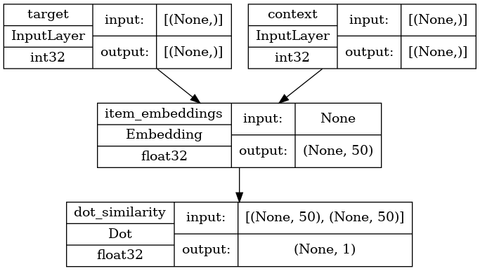
我們的 skip-gram 是一個簡單的二元分類模型,其運作方式如下:
- 會查詢
target電影的嵌入。 - 會查詢
context電影的嵌入。 - 在這兩個嵌入之間計算點積。
- 將結果 (在 sigmoid 激活後) 與標籤進行比較。
- 使用二元交叉熵損失。
learning_rate = 0.001
embedding_dim = 50
num_epochs = 10
實作模型
def create_model(vocabulary_size, embedding_dim):

    inputs = {
        "target": layers.Input(name="target", shape=(), dtype="int32"),
        "context": layers.Input(name="context", shape=(), dtype="int32"),
    }
    # Initialize item embeddings.
    embed_item = layers.Embedding(
        input_dim=vocabulary_size,
        output_dim=embedding_dim,
        embeddings_initializer="he_normal",
        embeddings_regularizer=keras.regularizers.l2(1e-6),
        name="item_embeddings",
    )
    # Lookup embeddings for target.
    target_embeddings = embed_item(inputs["target"])
    # Lookup embeddings for context.
    context_embeddings = embed_item(inputs["context"])
    # Compute dot similarity between target and context embeddings.
    logits = layers.Dot(axes=1, normalize=False, name="dot_similarity")(
        [target_embeddings, context_embeddings]
    )
    # Create the model.
    model = keras.Model(inputs=inputs, outputs=logits)
    return model
訓練模型
我們實例化模型並進行編譯。
model = create_model(len(vocabulary), embedding_dim)
model.compile(
    optimizer=keras.optimizers.Adam(learning_rate),
    loss=keras.losses.BinaryCrossentropy(from_logits=True),
)
讓我們繪製模型。
keras.utils.plot_model(
    model,
    show_shapes=True,
    show_dtype=True,
    show_layer_names=True,
)
現在,我們在 dataset 上訓練模型。
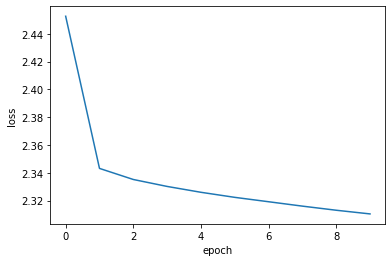
history = model.fit(dataset, epochs=num_epochs)
Epoch 1/10
860/860 [==============================] - 5s 5ms/step - loss: 2.4527
Epoch 2/10
860/860 [==============================] - 4s 5ms/step - loss: 2.3431
Epoch 3/10
860/860 [==============================] - 4s 4ms/step - loss: 2.3351
Epoch 4/10
860/860 [==============================] - 4s 4ms/step - loss: 2.3301
Epoch 5/10
860/860 [==============================] - 4s 5ms/step - loss: 2.3259
Epoch 6/10
860/860 [==============================] - 4s 4ms/step - loss: 2.3223
Epoch 7/10
860/860 [==============================] - 4s 5ms/step - loss: 2.3191
Epoch 8/10
860/860 [==============================] - 4s 4ms/step - loss: 2.3160
Epoch 9/10
860/860 [==============================] - 4s 4ms/step - loss: 2.3130
Epoch 10/10
860/860 [==============================] - 4s 5ms/step - loss: 2.3104
最後,我們繪製學習歷史。
plt.plot(history.history["loss"])
plt.ylabel("loss")
plt.xlabel("epoch")
plt.show()
分析學習到的嵌入。
movie_embeddings = model.get_layer("item_embeddings").get_weights()[0]
print("Embeddings shape:", movie_embeddings.shape)
Embeddings shape: (1406, 50)
尋找相關電影
定義包含一些名為 query_movies 的電影清單。
query_movies = [
    "Matrix, The (1999)",
    "Star Wars: Episode IV - A New Hope (1977)",
    "Lion King, The (1994)",
    "Terminator 2: Judgment Day (1991)",
    "Godfather, The (1972)",
]
取得 query_movies 中電影的嵌入。
query_embeddings = []

for movie_title in query_movies:
    movieId = get_movie_id_by_title(movie_title)
    token_id = vocabulary_lookup[movieId]
    movie_embedding = movie_embeddings[token_id]
    query_embeddings.append(movie_embedding)

query_embeddings = np.array(query_embeddings)
計算 query_movies 的嵌入與所有其他電影之間的 餘弦相似度,然後為每部電影選取前 k 個。
similarities = tf.linalg.matmul(
    tf.math.l2_normalize(query_embeddings),
    tf.math.l2_normalize(movie_embeddings),
    transpose_b=True,
)

_, indices = tf.math.top_k(similarities, k=5)
indices = indices.numpy().tolist()
顯示 query_movies 中前幾部相關電影。
for idx, title in enumerate(query_movies):
    print(title)
    print("".rjust(len(title), "-"))
    similar_tokens = indices[idx]
    for token in similar_tokens:
        similar_movieId = vocabulary[token]
        similar_title = get_movie_title_by_id(similar_movieId)
        print(f"- {similar_title}")
    print()
Matrix, The (1999)
------------------
- Matrix, The (1999)
- Raiders of the Lost Ark (Indiana Jones and the Raiders of the Lost Ark) (1981)
- Schindler's List (1993)
- Star Wars: Episode IV - A New Hope (1977)
- Lord of the Rings: The Fellowship of the Ring, The (2001)
Star Wars: Episode IV - A New Hope (1977)
-----------------------------------------
- Star Wars: Episode IV - A New Hope (1977)
- Schindler's List (1993)
- Raiders of the Lost Ark (Indiana Jones and the Raiders of the Lost Ark) (1981)
- Matrix, The (1999)
- Pulp Fiction (1994)
Lion King, The (1994)
---------------------
- Lion King, The (1994)
- Jurassic Park (1993)
- Independence Day (a.k.a. ID4) (1996)
- Beauty and the Beast (1991)
- Mrs. Doubtfire (1993)
Terminator 2: Judgment Day (1991)
---------------------------------
- Schindler's List (1993)
- Jurassic Park (1993)
- Terminator 2: Judgment Day (1991)
- Star Wars: Episode IV - A New Hope (1977)
- Back to the Future (1985)
Godfather, The (1972)
---------------------
- Apocalypse Now (1979)
- Fargo (1996)
- Godfather, The (1972)
- Schindler's List (1993)
- Casablanca (1942)
使用嵌入投影儀視覺化嵌入
import io

out_v = io.open("embeddings.tsv", "w", encoding="utf-8")
out_m = io.open("metadata.tsv", "w", encoding="utf-8")

for idx, movie_id in enumerate(vocabulary[1:]):
    movie_title = list(movies[movies.movieId == movie_id].title)[0]
    vector = movie_embeddings[idx]
    out_v.write("\t".join([str(x) for x in vector]) + "\n")
    out_m.write(movie_title + "\n")

out_v.close()
out_m.close()
下載 embeddings.tsv 和 metadata.tsv,以在 嵌入投影儀中分析取得的嵌入。
在 HuggingFace 上提供的範例
| 訓練的模型 | 示範 |
|---|---|