知識蒸餾方法
作者: Sayak Paul
建立日期 2021/08/01
上次修改 2021/08/01
說明:透過使用函數匹配進行知識蒸餾,訓練更好的學生模型。

簡介
知識蒸餾 (Hinton 等人) 是一種使我們能夠將較大型模型壓縮為較小型模型的技術。這使我們能夠在降低儲存和記憶體成本並實現更高的推論速度的同時,獲得高效能較大型模型的好處。
- 較小型模型 -> 較小的記憶體佔用空間
- 降低複雜度 -> 更少浮點運算 (FLOP)
在 知識蒸餾:好的教師是耐心且一致的 中,Beyer 等人研究了用於執行知識蒸餾的各種現有設定,並表明它們都會導致次佳效能。因此,實務人員在開發資源受限的生產系統時,通常會選擇其他替代方案 (量化、剪枝、權重叢集等)。
Beyer 等人研究了我們如何改進知識蒸餾過程產生的學生模型,並始終匹配其教師模型的效能。在這個範例中,我們將使用 Flowers102 資料集,研究他們介紹的方法。作為參考,使用這些方法,作者能夠產生一個在 ImageNet-1k 資料集上達到 82.8% 準確度的 ResNet50 模型。
如果您需要複習知識蒸餾,並想研究如何在 Keras 中實作知識蒸餾,您可以參考這個範例。您也可以遵循這個範例,其中顯示了知識蒸餾應用於一致性訓練的延伸。
若要遵循這個範例,您需要 TensorFlow 2.5 或更高版本,以及 TensorFlow Addons,可以使用以下命令安裝
!pip install -q tensorflow-addons
匯入
from tensorflow import keras
import tensorflow_addons as tfa
import tensorflow as tf

import matplotlib.pyplot as plt
import numpy as np

import tensorflow_datasets as tfds

tfds.disable_progress_bar()
超參數和常數
AUTO = tf.data.AUTOTUNE  # Used to dynamically adjust parallelism.
BATCH_SIZE = 64

# Comes from Table 4 and "Training setup" section.
TEMPERATURE = 10  # Used to soften the logits before they go to softmax.
INIT_LR = 0.003  # Initial learning rate that will be decayed over the training period.
WEIGHT_DECAY = 0.001  # Used for regularization.
CLIP_THRESHOLD = 1.0  # Used for clipping the gradients by L2-norm.

# We will first resize the training images to a bigger size and then we will take
# random crops of a lower size.
BIGGER = 160
RESIZE = 128
載入 Flowers102 資料集
train_ds, validation_ds, test_ds = tfds.load(
    "oxford_flowers102", split=["train", "validation", "test"], as_supervised=True
)
print(f"Number of training examples: {train_ds.cardinality()}.")
print(
    f"Number of validation examples: {validation_ds.cardinality()}."
)
print(f"Number of test examples: {test_ds.cardinality()}.")
Number of training examples: 1020.
Number of validation examples: 1020.
Number of test examples: 6149.
教師模型
與任何蒸餾技術一樣,重要的是首先訓練一個效能良好的教師模型,該模型通常大於後續的學生模型。作者將 BiT ResNet152x2 模型 (教師) 蒸餾到 BiT ResNet50 模型 (學生)。
BiT 代表 Big Transfer,是在 Big Transfer (BiT):通用視覺表示學習 中介紹的。ResNet 的 BiT 變體使用群組正規化 (Wu 等人) 和權重標準化 (Qiao 等人) 來取代批次正規化 (Ioffe 等人)。為了限制執行此範例所需的時間,我們將使用已在 Flowers102 資料集上訓練的 BiT ResNet101x3。您可以參考這個筆記本,以了解有關訓練過程的更多資訊。這個模型在 Flowers102 的測試集上達到 98.18% 的準確度。
模型權重託管在 Kaggle 上作為資料集。若要下載權重,請按照下列步驟操作
- 在 這裡 建立一個 Kaggle 帳戶。
- 前往您的使用者個人資料的「帳戶」標籤。
- 選取「建立 API 權杖」。這會觸發下載
kaggle.json,這是一個包含您 API 憑證的檔案。 - 從該 JSON 檔案中,複製您的 Kaggle 使用者名稱和 API 金鑰。
現在執行以下操作
import os

os.environ["KAGGLE_USERNAME"] = "" # TODO: enter your Kaggle user name here
os.environ["KAGGLE_KEY"] = "" # TODO: enter your Kaggle key here
設定環境變數後,執行
$ kaggle datasets download -d spsayakpaul/bitresnet101x3flowers102
$ unzip -qq bitresnet101x3flowers102.zip
這應該會產生一個名為 T-r101x3-128 的資料夾,這本質上是一個教師 SavedModel。
import os

os.environ["KAGGLE_USERNAME"] = ""  # TODO: enter your Kaggle user name here
os.environ["KAGGLE_KEY"] = ""  # TODO: enter your Kaggle API key here
!kaggle datasets download -d spsayakpaul/bitresnet101x3flowers102
!unzip -qq bitresnet101x3flowers102.zip
# Since the teacher model is not going to be trained further we make
# it non-trainable.
teacher_model = keras.models.load_model(
    "/home/jupyter/keras-io/examples/keras_recipes/T-r101x3-128"
)
teacher_model.trainable = False
teacher_model.summary()
Model: "my_bi_t_model_1"
_________________________________________________________________
Layer (type)                 Output Shape              Param #
=================================================================
dense_1 (Dense)              multiple                  626790
_________________________________________________________________
keras_layer_1 (KerasLayer)   multiple                  381789888
=================================================================
Total params: 382,416,678
Trainable params: 0
Non-trainable params: 382,416,678
_________________________________________________________________
「函數匹配」方法
為了訓練高品質的學生模型,作者建議對學生訓練工作流程進行以下變更
- 使用 MixUp 的激進變體 (Zhang 等人)。這是透過從均勻分佈而非 beta 分佈中取樣
alpha參數來完成的。MixUp 在此處使用,以幫助學生模型捕捉教師模型底層的函數。MixUp 在資料流形中不同樣本之間進行線性插值。因此,此處的基本原理是,如果訓練學生來擬合,它應該能夠更好地匹配教師模型。為了結合更多不變性,MixUp 與「Inception 式」裁剪 (Szegedy 等人) 相結合。這就是「函數匹配」術語在原始論文中出現的地方。 - 與其他著作 (例如 Noisy Student Training) 不同,教師和學生模型都收到同一張圖片副本,該圖片被混合和隨機裁剪。透過為兩個模型提供相同的輸入,作者使教師與學生保持一致。
- 使用 MixUp,我們在本質上是在訓練學生時引入了強烈的正規化形式。因此,它應該經過相對較長的時間訓練 (至少 1000 個 epoch)。由於學生在接受強烈正規化的訓練,因此由於較長的訓練排程而導致過度擬合的風險也得以降低。
總之,訓練學生模型時需要保持一致和耐心。
資料輸入管道
def mixup(images, labels):
    alpha = tf.random.uniform([], 0, 1)
    mixedup_images = alpha * images + (1 - alpha) * tf.reverse(images, axis=[0])
    # The labels do not matter here since they are NOT used during
    # training.
    return mixedup_images, labels


def preprocess_image(image, label, train=True):
    image = tf.cast(image, tf.float32) / 255.0

    if train:
        image = tf.image.resize(image, (BIGGER, BIGGER))
        image = tf.image.random_crop(image, (RESIZE, RESIZE, 3))
        image = tf.image.random_flip_left_right(image)
    else:
        # Central fraction amount is from here:
        # https://git.io/J8Kda.
        image = tf.image.central_crop(image, central_fraction=0.875)
        image = tf.image.resize(image, (RESIZE, RESIZE))

    return image, label


def prepare_dataset(dataset, train=True, batch_size=BATCH_SIZE):
    if train:
        dataset = dataset.map(preprocess_image, num_parallel_calls=AUTO)
        dataset = dataset.shuffle(BATCH_SIZE * 10)
    else:
        dataset = dataset.map(
            lambda x, y: (preprocess_image(x, y, train)), num_parallel_calls=AUTO
        )
    dataset = dataset.batch(batch_size)

    if train:
        dataset = dataset.map(mixup, num_parallel_calls=AUTO)

    dataset = dataset.prefetch(AUTO)
    return dataset
請注意,為簡潔起見,我們對訓練集使用了輕微裁剪,但在實務中應套用「Inception 式」預處理。您可以參考這個指令碼,以取得更接近的實作。此外,真實標籤不適用於訓練學生。
train_ds = prepare_dataset(train_ds, True)
validation_ds = prepare_dataset(validation_ds, False)
test_ds = prepare_dataset(test_ds, False)
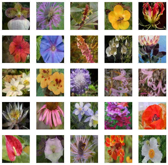
視覺化
sample_images, _ = next(iter(train_ds))
plt.figure(figsize=(10, 10))
for n in range(25):
    ax = plt.subplot(5, 5, n + 1)
    plt.imshow(sample_images[n].numpy())
    plt.axis("off")
plt.show()
學生模型
就本範例而言,我們將使用標準 ResNet50V2 (He 等人)。
def get_resnetv2():
    resnet_v2 = keras.applications.ResNet50V2(
        weights=None,
        input_shape=(RESIZE, RESIZE, 3),
        classes=102,
        classifier_activation="linear",
    )
    return resnet_v2


get_resnetv2().count_params()
23773798
與教師模型相比,此模型少了 3.58 億個參數。
蒸餾公用程式
我們將重複使用這個範例中關於知識蒸餾的一些程式碼。
class Distiller(tf.keras.Model):
    def __init__(self, student, teacher):
        super().__init__()
        self.student = student
        self.teacher = teacher
        self.loss_tracker = keras.metrics.Mean(name="distillation_loss")

    @property
    def metrics(self):
        metrics = super().metrics
        metrics.append(self.loss_tracker)
        return metrics

    def compile(
        self, optimizer, metrics, distillation_loss_fn, temperature=TEMPERATURE,
    ):
        super().compile(optimizer=optimizer, metrics=metrics)
        self.distillation_loss_fn = distillation_loss_fn
        self.temperature = temperature

    def train_step(self, data):
        # Unpack data
        x, _ = data

        # Forward pass of teacher
        teacher_predictions = self.teacher(x, training=False)

        with tf.GradientTape() as tape:
            # Forward pass of student
            student_predictions = self.student(x, training=True)

            # Compute loss
            distillation_loss = self.distillation_loss_fn(
                tf.nn.softmax(teacher_predictions / self.temperature, axis=1),
                tf.nn.softmax(student_predictions / self.temperature, axis=1),
            )

        # Compute gradients
        trainable_vars = self.student.trainable_variables
        gradients = tape.gradient(distillation_loss, trainable_vars)

        # Update weights
        self.optimizer.apply_gradients(zip(gradients, trainable_vars))

        # Report progress
        self.loss_tracker.update_state(distillation_loss)
        return {"distillation_loss": self.loss_tracker.result()}

    def test_step(self, data):
        # Unpack data
        x, y = data

        # Forward passes
        teacher_predictions = self.teacher(x, training=False)
        student_predictions = self.student(x, training=False)

        # Calculate the loss
        distillation_loss = self.distillation_loss_fn(
            tf.nn.softmax(teacher_predictions / self.temperature, axis=1),
            tf.nn.softmax(student_predictions / self.temperature, axis=1),
        )

        # Report progress
        self.loss_tracker.update_state(distillation_loss)
        self.compiled_metrics.update_state(y, student_predictions)
        results = {m.name: m.result() for m in self.metrics}
        return results
學習速率排程
論文中使用預熱餘弦學習速率排程。此排程對於許多預訓練方法 (尤其是電腦視覺) 也很常見。
# Some code is taken from:
# https://www.kaggle.com/ashusma/training-rfcx-tensorflow-tpu-effnet-b2.


class WarmUpCosine(keras.optimizers.schedules.LearningRateSchedule):
    def __init__(
        self, learning_rate_base, total_steps, warmup_learning_rate, warmup_steps
    ):
        super().__init__()

        self.learning_rate_base = learning_rate_base
        self.total_steps = total_steps
        self.warmup_learning_rate = warmup_learning_rate
        self.warmup_steps = warmup_steps
        self.pi = tf.constant(np.pi)

    def __call__(self, step):
        if self.total_steps < self.warmup_steps:
            raise ValueError("Total_steps must be larger or equal to warmup_steps.")

        cos_annealed_lr = tf.cos(
            self.pi
            * (tf.cast(step, tf.float32) - self.warmup_steps)
            / float(self.total_steps - self.warmup_steps)
        )
        learning_rate = 0.5 * self.learning_rate_base * (1 + cos_annealed_lr)

        if self.warmup_steps > 0:
            if self.learning_rate_base < self.warmup_learning_rate:
                raise ValueError(
                    "Learning_rate_base must be larger or equal to "
                    "warmup_learning_rate."
                )
            slope = (
                self.learning_rate_base - self.warmup_learning_rate
            ) / self.warmup_steps
            warmup_rate = slope * tf.cast(step, tf.float32) + self.warmup_learning_rate
            learning_rate = tf.where(
                step < self.warmup_steps, warmup_rate, learning_rate
            )
        return tf.where(
            step > self.total_steps, 0.0, learning_rate, name="learning_rate"
        )
我們現在可以繪製使用此排程產生的學習速率圖表。
ARTIFICIAL_EPOCHS = 1000
ARTIFICIAL_BATCH_SIZE = 512
DATASET_NUM_TRAIN_EXAMPLES = 1020
TOTAL_STEPS = int(
    DATASET_NUM_TRAIN_EXAMPLES / ARTIFICIAL_BATCH_SIZE * ARTIFICIAL_EPOCHS
)
scheduled_lrs = WarmUpCosine(
    learning_rate_base=INIT_LR,
    total_steps=TOTAL_STEPS,
    warmup_learning_rate=0.0,
    warmup_steps=1500,
)

lrs = [scheduled_lrs(step) for step in range(TOTAL_STEPS)]
plt.plot(lrs)
plt.xlabel("Step", fontsize=14)
plt.ylabel("LR", fontsize=14)
plt.show()
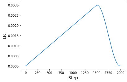
原始論文使用至少 1000 個 epoch 和 512 的批次大小來執行「函數匹配」。本範例的目的是呈現實作方法的流程,而不是展示在全面應用時的結果。但是,這些方法將轉移到論文中的原始設定。如果您有興趣了解更多資訊,請參閱此儲存庫。
訓練
optimizer = tfa.optimizers.AdamW(
    weight_decay=WEIGHT_DECAY, learning_rate=scheduled_lrs, clipnorm=CLIP_THRESHOLD
)

student_model = get_resnetv2()

distiller = Distiller(student=student_model, teacher=teacher_model)
distiller.compile(
    optimizer,
    metrics=[keras.metrics.SparseCategoricalAccuracy()],
    distillation_loss_fn=keras.losses.KLDivergence(),
    temperature=TEMPERATURE,
)

history = distiller.fit(
    train_ds,
    steps_per_epoch=int(np.ceil(DATASET_NUM_TRAIN_EXAMPLES / BATCH_SIZE)),
    validation_data=validation_ds,
    epochs=30,  # This should be at least 1000.
)

student = distiller.student
student_model.compile(metrics=["accuracy"])
_, top1_accuracy = student.evaluate(test_ds)
print(f"Top-1 accuracy on the test set: {round(top1_accuracy * 100, 2)}%")
Epoch 1/30
16/16 [==============================] - 74s 3s/step - distillation_loss: 0.0070 - val_sparse_categorical_accuracy: 0.0039 - val_distillation_loss: 0.0061
Epoch 2/30
16/16 [==============================] - 37s 2s/step - distillation_loss: 0.0059 - val_sparse_categorical_accuracy: 0.0098 - val_distillation_loss: 0.0061
Epoch 3/30
16/16 [==============================] - 37s 2s/step - distillation_loss: 0.0049 - val_sparse_categorical_accuracy: 0.0098 - val_distillation_loss: 0.0060
Epoch 4/30
16/16 [==============================] - 37s 2s/step - distillation_loss: 0.0048 - val_sparse_categorical_accuracy: 0.0098 - val_distillation_loss: 0.0060
Epoch 5/30
16/16 [==============================] - 37s 2s/step - distillation_loss: 0.0043 - val_sparse_categorical_accuracy: 0.0098 - val_distillation_loss: 0.0060
Epoch 6/30
16/16 [==============================] - 37s 2s/step - distillation_loss: 0.0041 - val_sparse_categorical_accuracy: 0.0108 - val_distillation_loss: 0.0060
Epoch 7/30
16/16 [==============================] - 37s 2s/step - distillation_loss: 0.0038 - val_sparse_categorical_accuracy: 0.0098 - val_distillation_loss: 0.0061
Epoch 8/30
16/16 [==============================] - 37s 2s/step - distillation_loss: 0.0040 - val_sparse_categorical_accuracy: 0.0098 - val_distillation_loss: 0.0062
Epoch 9/30
16/16 [==============================] - 37s 2s/step - distillation_loss: 0.0039 - val_sparse_categorical_accuracy: 0.0098 - val_distillation_loss: 0.0063
Epoch 10/30
16/16 [==============================] - 37s 2s/step - distillation_loss: 0.0035 - val_sparse_categorical_accuracy: 0.0098 - val_distillation_loss: 0.0064
Epoch 11/30
16/16 [==============================] - 37s 2s/step - distillation_loss: 0.0041 - val_sparse_categorical_accuracy: 0.0098 - val_distillation_loss: 0.0064
Epoch 12/30
16/16 [==============================] - 37s 2s/step - distillation_loss: 0.0039 - val_sparse_categorical_accuracy: 0.0098 - val_distillation_loss: 0.0067
Epoch 13/30
16/16 [==============================] - 37s 2s/step - distillation_loss: 0.0039 - val_sparse_categorical_accuracy: 0.0098 - val_distillation_loss: 0.0067
Epoch 14/30
16/16 [==============================] - 37s 2s/step - distillation_loss: 0.0036 - val_sparse_categorical_accuracy: 0.0098 - val_distillation_loss: 0.0066
Epoch 15/30
16/16 [==============================] - 37s 2s/step - distillation_loss: 0.0037 - val_sparse_categorical_accuracy: 0.0098 - val_distillation_loss: 0.0065
Epoch 16/30
16/16 [==============================] - 37s 2s/step - distillation_loss: 0.0038 - val_sparse_categorical_accuracy: 0.0098 - val_distillation_loss: 0.0068
Epoch 17/30
16/16 [==============================] - 37s 2s/step - distillation_loss: 0.0039 - val_sparse_categorical_accuracy: 0.0098 - val_distillation_loss: 0.0066
Epoch 18/30
16/16 [==============================] - 37s 2s/step - distillation_loss: 0.0038 - val_sparse_categorical_accuracy: 0.0098 - val_distillation_loss: 0.0064
Epoch 19/30
16/16 [==============================] - 37s 2s/step - distillation_loss: 0.0035 - val_sparse_categorical_accuracy: 0.0098 - val_distillation_loss: 0.0071
Epoch 20/30
16/16 [==============================] - 37s 2s/step - distillation_loss: 0.0038 - val_sparse_categorical_accuracy: 0.0098 - val_distillation_loss: 0.0066
Epoch 21/30
16/16 [==============================] - 37s 2s/step - distillation_loss: 0.0038 - val_sparse_categorical_accuracy: 0.0098 - val_distillation_loss: 0.0068
Epoch 22/30
16/16 [==============================] - 37s 2s/step - distillation_loss: 0.0034 - val_sparse_categorical_accuracy: 0.0098 - val_distillation_loss: 0.0073
Epoch 23/30
16/16 [==============================] - 37s 2s/step - distillation_loss: 0.0035 - val_sparse_categorical_accuracy: 0.0098 - val_distillation_loss: 0.0078
Epoch 24/30
16/16 [==============================] - 37s 2s/step - distillation_loss: 0.0037 - val_sparse_categorical_accuracy: 0.0098 - val_distillation_loss: 0.0087
Epoch 25/30
16/16 [==============================] - 37s 2s/step - distillation_loss: 0.0031 - val_sparse_categorical_accuracy: 0.0108 - val_distillation_loss: 0.0078
Epoch 26/30
16/16 [==============================] - 37s 2s/step - distillation_loss: 0.0033 - val_sparse_categorical_accuracy: 0.0098 - val_distillation_loss: 0.0072
Epoch 27/30
16/16 [==============================] - 37s 2s/step - distillation_loss: 0.0036 - val_sparse_categorical_accuracy: 0.0098 - val_distillation_loss: 0.0071
Epoch 28/30
16/16 [==============================] - 37s 2s/step - distillation_loss: 0.0036 - val_sparse_categorical_accuracy: 0.0275 - val_distillation_loss: 0.0078
Epoch 29/30
16/16 [==============================] - 37s 2s/step - distillation_loss: 0.0032 - val_sparse_categorical_accuracy: 0.0196 - val_distillation_loss: 0.0068
Epoch 30/30
16/16 [==============================] - 37s 2s/step - distillation_loss: 0.0034 - val_sparse_categorical_accuracy: 0.0147 - val_distillation_loss: 0.0071
97/97 [==============================] - 7s 64ms/step - loss: 0.0000e+00 - accuracy: 0.0107
Top-1 accuracy on the test set: 1.07%
結果
僅經過 30 個 epoch 的訓練,結果遠未達到預期。這就是耐心 (也就是較長的訓練排程) 的好處將發揮作用的地方。讓我們調查一下經過 1000 個 epoch 訓練的模型可以做什麼。
# Download the pre-trained weights.
!wget https://git.io/JBO3Y -O S-r50x1-128-1000.tar.gz
!tar xf S-r50x1-128-1000.tar.gz
pretrained_student = keras.models.load_model("S-r50x1-128-1000")
pretrained_student.summary()
Model: "resnet"
_________________________________________________________________
Layer (type)                 Output Shape              Param #
=================================================================
root_block (Sequential)      (None, 32, 32, 64)        9408
_________________________________________________________________
block1 (Sequential)          (None, 32, 32, 256)       214912
_________________________________________________________________
block2 (Sequential)          (None, 16, 16, 512)       1218048
_________________________________________________________________
block3 (Sequential)          (None, 8, 8, 1024)        7095296
_________________________________________________________________
block4 (Sequential)          (None, 4, 4, 2048)        14958592
_________________________________________________________________
group_norm (GroupNormalizati multiple                  4096
_________________________________________________________________
re_lu_97 (ReLU)              multiple                  0
_________________________________________________________________
global_average_pooling2d_1 ( multiple                  0
_________________________________________________________________
head/dense (Dense)           multiple                  208998
=================================================================
Total params: 23,709,350
Trainable params: 23,709,350
Non-trainable params: 0
_________________________________________________________________
這個模型完全遵循作者在他們的學生模型中使用的內容。這就是為什麼模型摘要有點不同的原因。
_, top1_accuracy = pretrained_student.evaluate(test_ds)
print(f"Top-1 accuracy on the test set: {round(top1_accuracy * 100, 2)}%")
97/97 [==============================] - 14s 131ms/step - loss: 0.0000e+00 - accuracy: 0.8102
Top-1 accuracy on the test set: 81.02%
經過 100,000 個 epoch 的訓練,這個相同的模型可產生 95.54% 的 top-1 準確度。
論文中介紹了一些重要的消融研究,這些研究顯示了與先前技術相比,這些方法的有效性。因此,如果您對這些方法持懷疑態度,請務必參考論文。
關於較長時間訓練的注意事項
使用基於 TPU 的硬體基礎結構,我們可以更快地訓練模型 1000 個 epoch。這甚至不需要對此程式碼庫進行大量變更。建議您查看此儲存庫,因為它提供了這些方法的 TPU 相容訓練流程,並且可以在Kaggle 核心上執行,利用他們免費的 TPU v3-8 硬體。