Keras 除錯技巧
作者: fchollet
建立日期 2020/05/16
上次修改日期 2023/11/16
說明: 四個簡單的技巧,可協助您除錯 Keras 程式碼。

簡介
一般來說,在 Keras 中幾乎可以不用編寫程式碼來完成任何事情:無論您是要實作新的 GAN 類型,還是用於影像分割的最新卷積網路架構,您通常都可以堅持呼叫內建方法。由於所有內建方法都會執行廣泛的輸入驗證檢查,因此您幾乎不需要進行任何除錯。完全由內建層組成的 Functional API 模型會在第一次嘗試時就可運作 – 如果您可以編譯它,它就會執行。
但是,有時您需要深入研究並編寫自己的程式碼。以下是一些常見的範例
- 建立新的
Layer子類別。 - 建立自訂
Metric子類別。 - 在
Model上實作自訂train_step。
此文件提供一些簡單的技巧,可協助您在這些情況下進行除錯。
技巧 1:在測試整體之前先測試每個部分
如果您建立的任何物件有可能無法如預期運作,請不要只是將其放入端對端程序中並觀察火花四射。而是先隔離測試您的自訂物件。這似乎很明顯 – 但您會驚訝地發現有多少人沒有從這裡開始。
- 如果您編寫自訂層,請不要立即對整個模型呼叫
fit()。先在一些測試資料上呼叫您的層。 - 如果您編寫自訂指標,請先列印一些參考輸入的輸出。
這是一個簡單的範例。讓我們編寫一個含有錯誤的自訂層
import os

# The last example uses tf.GradientTape and thus requires TensorFlow.
# However, all tips here are applicable with all backends.
os.environ["KERAS_BACKEND"] = "tensorflow"

import keras
from keras import layers
from keras import ops
import numpy as np
import tensorflow as tf


class MyAntirectifier(layers.Layer):
    def build(self, input_shape):
        output_dim = input_shape[-1]
        self.kernel = self.add_weight(
            shape=(output_dim * 2, output_dim),
            initializer="he_normal",
            name="kernel",
            trainable=True,
        )

    def call(self, inputs):
        # Take the positive part of the input
        pos = ops.relu(inputs)
        # Take the negative part of the input
        neg = ops.relu(-inputs)
        # Concatenate the positive and negative parts
        concatenated = ops.concatenate([pos, neg], axis=0)
        # Project the concatenation down to the same dimensionality as the input
        return ops.matmul(concatenated, self.kernel)
現在,不要直接在端對端模型中使用它,而是嘗試在一些測試資料上呼叫該層
x = tf.random.normal(shape=(2, 5))
y = MyAntirectifier()(x)
我們得到以下錯誤
...
      1 x = tf.random.normal(shape=(2, 5))
----> 2 y = MyAntirectifier()(x)
...
     17         neg = tf.nn.relu(-inputs)
     18         concatenated = tf.concat([pos, neg], axis=0)
---> 19         return tf.matmul(concatenated, self.kernel)
...
InvalidArgumentError: Matrix size-incompatible: In[0]: [4,5], In[1]: [10,5] [Op:MatMul]
看來 matmul 運算中的輸入張量可能具有不正確的形狀。讓我們新增列印陳述式來檢查實際形狀
class MyAntirectifier(layers.Layer):
    def build(self, input_shape):
        output_dim = input_shape[-1]
        self.kernel = self.add_weight(
            shape=(output_dim * 2, output_dim),
            initializer="he_normal",
            name="kernel",
            trainable=True,
        )

    def call(self, inputs):
        pos = ops.relu(inputs)
        neg = ops.relu(-inputs)
        print("pos.shape:", pos.shape)
        print("neg.shape:", neg.shape)
        concatenated = ops.concatenate([pos, neg], axis=0)
        print("concatenated.shape:", concatenated.shape)
        print("kernel.shape:", self.kernel.shape)
        return ops.matmul(concatenated, self.kernel)
我們得到以下結果
pos.shape: (2, 5)
neg.shape: (2, 5)
concatenated.shape: (4, 5)
kernel.shape: (10, 5)
結果發現我們 concat 運算的軸錯誤!我們應該沿著特徵軸 1 而不是批次軸 0 連接 neg 和 pos。以下是正確的版本
class MyAntirectifier(layers.Layer):
    def build(self, input_shape):
        output_dim = input_shape[-1]
        self.kernel = self.add_weight(
            shape=(output_dim * 2, output_dim),
            initializer="he_normal",
            name="kernel",
            trainable=True,
        )

    def call(self, inputs):
        pos = ops.relu(inputs)
        neg = ops.relu(-inputs)
        print("pos.shape:", pos.shape)
        print("neg.shape:", neg.shape)
        concatenated = ops.concatenate([pos, neg], axis=1)
        print("concatenated.shape:", concatenated.shape)
        print("kernel.shape:", self.kernel.shape)
        return ops.matmul(concatenated, self.kernel)
現在我們的程式碼可以正常運作了
x = keras.random.normal(shape=(2, 5))
y = MyAntirectifier()(x)
pos.shape: (2, 5)
neg.shape: (2, 5)
concatenated.shape: (2, 10)
kernel.shape: (10, 5)
技巧 2:使用 model.summary() 和 plot_model() 來檢查層的輸出形狀
如果您正在處理複雜的網路拓撲,您將需要一種方法來視覺化層的連接方式,以及它們如何轉換通過它們的資料。
這是一個範例。考慮這個具有三個輸入和兩個輸出的模型(取自 Functional API 指南)
num_tags = 12  # Number of unique issue tags
num_words = 10000  # Size of vocabulary obtained when preprocessing text data
num_departments = 4  # Number of departments for predictions

title_input = keras.Input(
    shape=(None,), name="title"
)  # Variable-length sequence of ints
body_input = keras.Input(shape=(None,), name="body")  # Variable-length sequence of ints
tags_input = keras.Input(
    shape=(num_tags,), name="tags"
)  # Binary vectors of size `num_tags`

# Embed each word in the title into a 64-dimensional vector
title_features = layers.Embedding(num_words, 64)(title_input)
# Embed each word in the text into a 64-dimensional vector
body_features = layers.Embedding(num_words, 64)(body_input)

# Reduce sequence of embedded words in the title into a single 128-dimensional vector
title_features = layers.LSTM(128)(title_features)
# Reduce sequence of embedded words in the body into a single 32-dimensional vector
body_features = layers.LSTM(32)(body_features)

# Merge all available features into a single large vector via concatenation
x = layers.concatenate([title_features, body_features, tags_input])

# Stick a logistic regression for priority prediction on top of the features
priority_pred = layers.Dense(1, name="priority")(x)
# Stick a department classifier on top of the features
department_pred = layers.Dense(num_departments, name="department")(x)

# Instantiate an end-to-end model predicting both priority and department
model = keras.Model(
    inputs=[title_input, body_input, tags_input],
    outputs=[priority_pred, department_pred],
)
呼叫 summary() 可以協助您檢查每個層的輸出形狀
model.summary()
Model: "functional_1"
┏━━━━━━━━━━━━━━━━━━━━━┳━━━━━━━━━━━━━━━━━━━┳━━━━━━━━━┳━━━━━━━━━━━━━━━━━━━━━━┓
┃ Layer (type)        ┃ Output Shape      ┃ Param # ┃ Connected to         ┃
┡━━━━━━━━━━━━━━━━━━━━━╇━━━━━━━━━━━━━━━━━━━╇━━━━━━━━━╇━━━━━━━━━━━━━━━━━━━━━━┩
│ title (InputLayer)  │ (None, None)      │       0 │ -                    │
├─────────────────────┼───────────────────┼─────────┼──────────────────────┤
│ body (InputLayer)   │ (None, None)      │       0 │ -                    │
├─────────────────────┼───────────────────┼─────────┼──────────────────────┤
│ embedding           │ (None, None, 64)  │ 640,000 │ title[0][0]          │
│ (Embedding)         │                   │         │                      │
├─────────────────────┼───────────────────┼─────────┼──────────────────────┤
│ embedding_1         │ (None, None, 64)  │ 640,000 │ body[0][0]           │
│ (Embedding)         │                   │         │                      │
├─────────────────────┼───────────────────┼─────────┼──────────────────────┤
│ lstm (LSTM)         │ (None, 128)       │  98,816 │ embedding[0][0]      │
├─────────────────────┼───────────────────┼─────────┼──────────────────────┤
│ lstm_1 (LSTM)       │ (None, 32)        │  12,416 │ embedding_1[0][0]    │
├─────────────────────┼───────────────────┼─────────┼──────────────────────┤
│ tags (InputLayer)   │ (None, 12)        │       0 │ -                    │
├─────────────────────┼───────────────────┼─────────┼──────────────────────┤
│ concatenate         │ (None, 172)       │       0 │ lstm[0][0],          │
│ (Concatenate)       │                   │         │ lstm_1[0][0],        │
│                     │                   │         │ tags[0][0]           │
├─────────────────────┼───────────────────┼─────────┼──────────────────────┤
│ priority (Dense)    │ (None, 1)         │     173 │ concatenate[0][0]    │
├─────────────────────┼───────────────────┼─────────┼──────────────────────┤
│ department (Dense)  │ (None, 4)         │     692 │ concatenate[0][0]    │
└─────────────────────┴───────────────────┴─────────┴──────────────────────┘
Total params: 1,392,097 (5.31 MB)
Trainable params: 1,392,097 (5.31 MB)
Non-trainable params: 0 (0.00 B)
您也可以使用 plot_model 視覺化整個網路拓撲以及輸出形狀
keras.utils.plot_model(model, show_shapes=True)
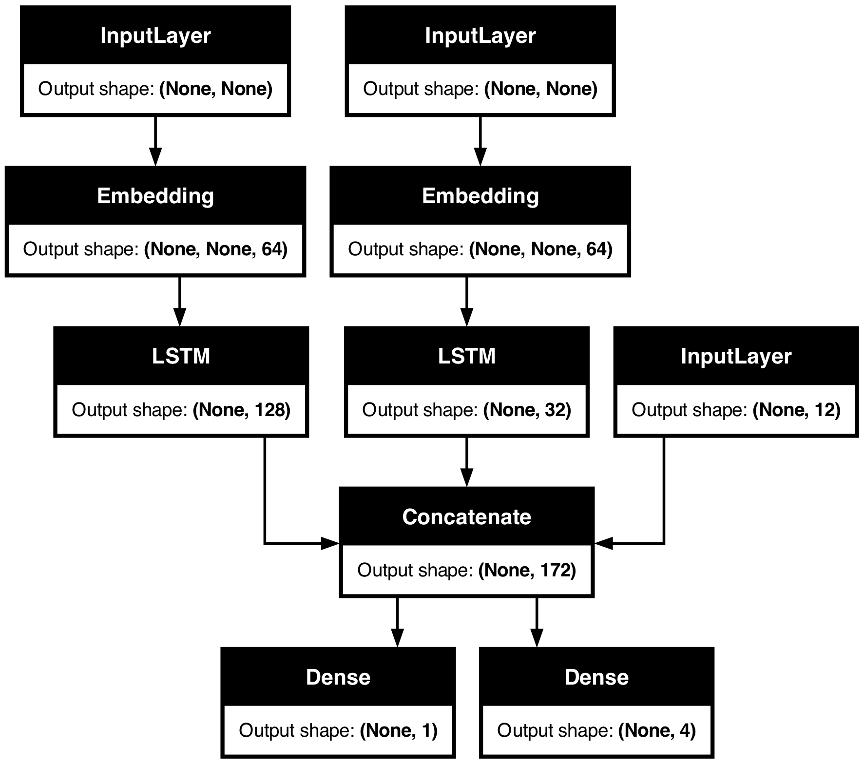
透過此圖,任何連線層級錯誤都會立即顯現出來。
技巧 3:要除錯 fit() 期間發生的情況,請使用 run_eagerly=True
fit() 方法速度很快:它會執行經過良好最佳化、完全編譯的計算圖。這對於效能來說很好,但也表示您正在執行的程式碼不是您編寫的 Python 程式碼。這在除錯時可能會出現問題。您可能還記得,Python 速度很慢 – 因此我們將其用作臨時語言,而不是執行語言。
幸好,有一種簡單的方法可以完全急切地在「除錯模式」中執行程式碼:將 run_eagerly=True 傳遞給 compile()。您對 fit() 的呼叫現在將逐行執行,而無需任何最佳化。它速度較慢,但可以列印中間張量的值,或使用 Python 除錯工具。非常適合除錯。
這是一個基本範例:讓我們編寫一個非常簡單的模型,其中包含自訂 train_step() 方法。我們的模型僅實作梯度下降,但它使用一階和二階梯度的組合,而不是一階梯度。到目前為止都很簡單。
您可以發現我們做錯了什麼嗎?
class MyModel(keras.Model):
    def train_step(self, data):
        inputs, targets = data
        trainable_vars = self.trainable_variables
        with tf.GradientTape() as tape2:
            with tf.GradientTape() as tape1:
                y_pred = self(inputs, training=True)  # Forward pass
                # Compute the loss value
                # (the loss function is configured in `compile()`)
                loss = self.compute_loss(y=targets, y_pred=y_pred)
            # Compute first-order gradients
            dl_dw = tape1.gradient(loss, trainable_vars)
        # Compute second-order gradients
        d2l_dw2 = tape2.gradient(dl_dw, trainable_vars)

        # Combine first-order and second-order gradients
        grads = [0.5 * w1 + 0.5 * w2 for (w1, w2) in zip(d2l_dw2, dl_dw)]

        # Update weights
        self.optimizer.apply_gradients(zip(grads, trainable_vars))

        # Update metrics (includes the metric that tracks the loss)
        for metric in self.metrics:
            if metric.name == "loss":
                metric.update_state(loss)
            else:
                metric.update_state(targets, y_pred)

        # Return a dict mapping metric names to current value
        return {m.name: m.result() for m in self.metrics}
讓我們使用此自訂損失函數在 MNIST 上訓練單層模型。
我們隨機選擇批次大小 1024 和學習率 0.1。一般概念是使用比平常更大的批次和更大的學習率,因為我們「改良」的梯度應可引導我們更快收斂。
# Construct an instance of MyModel
def get_model():
    inputs = keras.Input(shape=(784,))
    intermediate = layers.Dense(256, activation="relu")(inputs)
    outputs = layers.Dense(10, activation="softmax")(intermediate)
    model = MyModel(inputs, outputs)
    return model


# Prepare data
(x_train, y_train), _ = keras.datasets.mnist.load_data()
x_train = np.reshape(x_train, (-1, 784)) / 255

model = get_model()
model.compile(
    optimizer=keras.optimizers.SGD(learning_rate=1e-2),
    loss="sparse_categorical_crossentropy",
)
model.fit(x_train, y_train, epochs=3, batch_size=1024, validation_split=0.1)
Epoch 1/3
 53/53 ━━━━━━━━━━━━━━━━━━━━ 0s 7ms/step - loss: 2.4264 - val_loss: 2.3036
Epoch 2/3
 53/53 ━━━━━━━━━━━━━━━━━━━━ 0s 6ms/step - loss: 2.3111 - val_loss: 2.3387
Epoch 3/3
 53/53 ━━━━━━━━━━━━━━━━━━━━ 0s 7ms/step - loss: 2.3442 - val_loss: 2.3697

<keras.src.callbacks.history.History at 0x29a899600>
糟了,它沒有收斂!有些地方不盡如人意。
現在是逐步列印梯度情況的時候了。
我們在 train_step 方法中新增各種 print 陳述式,並確保將 run_eagerly=True 傳遞給 compile() 以逐步、急切地執行我們的程式碼。
class MyModel(keras.Model):
    def train_step(self, data):
        print()
        print("----Start of step: %d" % (self.step_counter,))
        self.step_counter += 1

        inputs, targets = data
        trainable_vars = self.trainable_variables
        with tf.GradientTape() as tape2:
            with tf.GradientTape() as tape1:
                y_pred = self(inputs, training=True)  # Forward pass
                # Compute the loss value
                # (the loss function is configured in `compile()`)
                loss = self.compute_loss(y=targets, y_pred=y_pred)
            # Compute first-order gradients
            dl_dw = tape1.gradient(loss, trainable_vars)
        # Compute second-order gradients
        d2l_dw2 = tape2.gradient(dl_dw, trainable_vars)

        print("Max of dl_dw[0]: %.4f" % tf.reduce_max(dl_dw[0]))
        print("Min of dl_dw[0]: %.4f" % tf.reduce_min(dl_dw[0]))
        print("Mean of dl_dw[0]: %.4f" % tf.reduce_mean(dl_dw[0]))
        print("-")
        print("Max of d2l_dw2[0]: %.4f" % tf.reduce_max(d2l_dw2[0]))
        print("Min of d2l_dw2[0]: %.4f" % tf.reduce_min(d2l_dw2[0]))
        print("Mean of d2l_dw2[0]: %.4f" % tf.reduce_mean(d2l_dw2[0]))

        # Combine first-order and second-order gradients
        grads = [0.5 * w1 + 0.5 * w2 for (w1, w2) in zip(d2l_dw2, dl_dw)]

        # Update weights
        self.optimizer.apply_gradients(zip(grads, trainable_vars))

        # Update metrics (includes the metric that tracks the loss)
        for metric in self.metrics:
            if metric.name == "loss":
                metric.update_state(loss)
            else:
                metric.update_state(targets, y_pred)

        # Return a dict mapping metric names to current value
        return {m.name: m.result() for m in self.metrics}


model = get_model()
model.compile(
    optimizer=keras.optimizers.SGD(learning_rate=1e-2),
    loss="sparse_categorical_crossentropy",
    metrics=["sparse_categorical_accuracy"],
    run_eagerly=True,
)
model.step_counter = 0
# We pass epochs=1 and steps_per_epoch=10 to only run 10 steps of training.
model.fit(x_train, y_train, epochs=1, batch_size=1024, verbose=0, steps_per_epoch=10)
----Start of step: 0
Max of dl_dw[0]: 0.0332
Min of dl_dw[0]: -0.0288
Mean of dl_dw[0]: 0.0003
-
Max of d2l_dw2[0]: 5.2691
Min of d2l_dw2[0]: -2.6968
Mean of d2l_dw2[0]: 0.0981
----Start of step: 1
Max of dl_dw[0]: 0.0445
Min of dl_dw[0]: -0.0169
Mean of dl_dw[0]: 0.0013
-
Max of d2l_dw2[0]: 3.3575
Min of d2l_dw2[0]: -1.9024
Mean of d2l_dw2[0]: 0.0726
----Start of step: 2
Max of dl_dw[0]: 0.0669
Min of dl_dw[0]: -0.0153
Mean of dl_dw[0]: 0.0013
-
Max of d2l_dw2[0]: 5.0661
Min of d2l_dw2[0]: -1.7168
Mean of d2l_dw2[0]: 0.0809
----Start of step: 3
Max of dl_dw[0]: 0.0545
Min of dl_dw[0]: -0.0125
Mean of dl_dw[0]: 0.0008
-
Max of d2l_dw2[0]: 6.5223
Min of d2l_dw2[0]: -0.6604
Mean of d2l_dw2[0]: 0.0991
----Start of step: 4
Max of dl_dw[0]: 0.0247
Min of dl_dw[0]: -0.0152
Mean of dl_dw[0]: -0.0001
-
Max of d2l_dw2[0]: 2.8030
Min of d2l_dw2[0]: -0.1156
Mean of d2l_dw2[0]: 0.0321
----Start of step: 5
Max of dl_dw[0]: 0.0051
Min of dl_dw[0]: -0.0096
Mean of dl_dw[0]: -0.0001
-
Max of d2l_dw2[0]: 0.2545
Min of d2l_dw2[0]: -0.0284
Mean of d2l_dw2[0]: 0.0079
----Start of step: 6
Max of dl_dw[0]: 0.0041
Min of dl_dw[0]: -0.0102
Mean of dl_dw[0]: -0.0001
-
Max of d2l_dw2[0]: 0.2198
Min of d2l_dw2[0]: -0.0175
Mean of d2l_dw2[0]: 0.0069
----Start of step: 7
Max of dl_dw[0]: 0.0035
Min of dl_dw[0]: -0.0086
Mean of dl_dw[0]: -0.0001
-
Max of d2l_dw2[0]: 0.1485
Min of d2l_dw2[0]: -0.0175
Mean of d2l_dw2[0]: 0.0060
----Start of step: 8
Max of dl_dw[0]: 0.0039
Min of dl_dw[0]: -0.0094
Mean of dl_dw[0]: -0.0001
-
Max of d2l_dw2[0]: 0.1454
Min of d2l_dw2[0]: -0.0130
Mean of d2l_dw2[0]: 0.0061
----Start of step: 9
Max of dl_dw[0]: 0.0028
Min of dl_dw[0]: -0.0087
Mean of dl_dw[0]: -0.0001
-
Max of d2l_dw2[0]: 0.1491
Min of d2l_dw2[0]: -0.0326
Mean of d2l_dw2[0]: 0.0058

<keras.src.callbacks.history.History at 0x2a0d1e440>
我們學到了什麼?
- 一階和二階梯度的值可能相差數個數量級。
- 有時,它們甚至可能沒有相同的符號。
- 它們的值在每個步驟可能會差異很大。
這引導我們得出一個顯而易見的想法:讓我們在組合梯度之前對它們進行正規化。
class MyModel(keras.Model):
    def train_step(self, data):
        inputs, targets = data
        trainable_vars = self.trainable_variables
        with tf.GradientTape() as tape2:
            with tf.GradientTape() as tape1:
                y_pred = self(inputs, training=True)  # Forward pass
                # Compute the loss value
                # (the loss function is configured in `compile()`)
                loss = self.compute_loss(y=targets, y_pred=y_pred)
            # Compute first-order gradients
            dl_dw = tape1.gradient(loss, trainable_vars)
        # Compute second-order gradients
        d2l_dw2 = tape2.gradient(dl_dw, trainable_vars)

        dl_dw = [tf.math.l2_normalize(w) for w in dl_dw]
        d2l_dw2 = [tf.math.l2_normalize(w) for w in d2l_dw2]

        # Combine first-order and second-order gradients
        grads = [0.5 * w1 + 0.5 * w2 for (w1, w2) in zip(d2l_dw2, dl_dw)]

        # Update weights
        self.optimizer.apply_gradients(zip(grads, trainable_vars))

        # Update metrics (includes the metric that tracks the loss)
        for metric in self.metrics:
            if metric.name == "loss":
                metric.update_state(loss)
            else:
                metric.update_state(targets, y_pred)

        # Return a dict mapping metric names to current value
        return {m.name: m.result() for m in self.metrics}


model = get_model()
model.compile(
    optimizer=keras.optimizers.SGD(learning_rate=1e-2),
    loss="sparse_categorical_crossentropy",
    metrics=["sparse_categorical_accuracy"],
)
model.fit(x_train, y_train, epochs=5, batch_size=1024, validation_split=0.1)
Epoch 1/5
 53/53 ━━━━━━━━━━━━━━━━━━━━ 1s 7ms/step - sparse_categorical_accuracy: 0.1250 - loss: 2.3185 - val_loss: 2.0502 - val_sparse_categorical_accuracy: 0.3373
Epoch 2/5
 53/53 ━━━━━━━━━━━━━━━━━━━━ 0s 6ms/step - sparse_categorical_accuracy: 0.3966 - loss: 1.9934 - val_loss: 1.8032 - val_sparse_categorical_accuracy: 0.5698
Epoch 3/5
 53/53 ━━━━━━━━━━━━━━━━━━━━ 0s 7ms/step - sparse_categorical_accuracy: 0.5663 - loss: 1.7784 - val_loss: 1.6241 - val_sparse_categorical_accuracy: 0.6470
Epoch 4/5
 53/53 ━━━━━━━━━━━━━━━━━━━━ 0s 7ms/step - sparse_categorical_accuracy: 0.6135 - loss: 1.6256 - val_loss: 1.5010 - val_sparse_categorical_accuracy: 0.6595
Epoch 5/5
 53/53 ━━━━━━━━━━━━━━━━━━━━ 0s 7ms/step - sparse_categorical_accuracy: 0.6216 - loss: 1.5173 - val_loss: 1.4169 - val_sparse_categorical_accuracy: 0.6625

<keras.src.callbacks.history.History at 0x2a0d4c640>
現在,訓練收斂了!它一點也不好用,但至少模型學到了一些東西。
在花費幾分鐘調整參數後,我們得到了以下運作良好的配置(達到 97% 的驗證準確度,並且似乎對過度擬合具有相當的穩健性)
- 使用
0.2 * w1 + 0.8 * w2來組合梯度。 - 使用隨著時間線性衰減的學習率。
我不會說這個想法行得通 – 這根本不是您應該如何進行二階最佳化(提示:請參閱牛頓法和高斯-牛頓法、準牛頓法和 BFGS)。但希望此示範可讓您了解如何從不舒服的訓練情況中除錯。
請記住:使用 run_eagerly=True 來除錯 fit() 中發生的情況。當您的程式碼終於如預期運作時,請務必移除此旗標,以便獲得最佳執行效能!
這是我們最終的訓練執行
class MyModel(keras.Model):
    def train_step(self, data):
        inputs, targets = data
        trainable_vars = self.trainable_variables
        with tf.GradientTape() as tape2:
            with tf.GradientTape() as tape1:
                y_pred = self(inputs, training=True)  # Forward pass
                # Compute the loss value
                # (the loss function is configured in `compile()`)
                loss = self.compute_loss(y=targets, y_pred=y_pred)
            # Compute first-order gradients
            dl_dw = tape1.gradient(loss, trainable_vars)
        # Compute second-order gradients
        d2l_dw2 = tape2.gradient(dl_dw, trainable_vars)

        dl_dw = [tf.math.l2_normalize(w) for w in dl_dw]
        d2l_dw2 = [tf.math.l2_normalize(w) for w in d2l_dw2]

        # Combine first-order and second-order gradients
        grads = [0.2 * w1 + 0.8 * w2 for (w1, w2) in zip(d2l_dw2, dl_dw)]

        # Update weights
        self.optimizer.apply_gradients(zip(grads, trainable_vars))

        # Update metrics (includes the metric that tracks the loss)
        for metric in self.metrics:
            if metric.name == "loss":
                metric.update_state(loss)
            else:
                metric.update_state(targets, y_pred)

        # Return a dict mapping metric names to current value
        return {m.name: m.result() for m in self.metrics}


model = get_model()
lr = learning_rate = keras.optimizers.schedules.InverseTimeDecay(
    initial_learning_rate=0.1, decay_steps=25, decay_rate=0.1
)
model.compile(
    optimizer=keras.optimizers.SGD(lr),
    loss="sparse_categorical_crossentropy",
    metrics=["sparse_categorical_accuracy"],
)
model.fit(x_train, y_train, epochs=50, batch_size=2048, validation_split=0.1)
Epoch 1/50
 27/27 ━━━━━━━━━━━━━━━━━━━━ 1s 14ms/step - sparse_categorical_accuracy: 0.5056 - loss: 1.7508 - val_loss: 0.6378 - val_sparse_categorical_accuracy: 0.8658
Epoch 2/50
 27/27 ━━━━━━━━━━━━━━━━━━━━ 0s 10ms/step - sparse_categorical_accuracy: 0.8407 - loss: 0.6323 - val_loss: 0.4039 - val_sparse_categorical_accuracy: 0.8970
Epoch 3/50
 27/27 ━━━━━━━━━━━━━━━━━━━━ 0s 10ms/step - sparse_categorical_accuracy: 0.8807 - loss: 0.4472 - val_loss: 0.3243 - val_sparse_categorical_accuracy: 0.9120
Epoch 4/50
 27/27 ━━━━━━━━━━━━━━━━━━━━ 0s 10ms/step - sparse_categorical_accuracy: 0.8947 - loss: 0.3781 - val_loss: 0.2861 - val_sparse_categorical_accuracy: 0.9235
Epoch 5/50
 27/27 ━━━━━━━━━━━━━━━━━━━━ 0s 11ms/step - sparse_categorical_accuracy: 0.9022 - loss: 0.3453 - val_loss: 0.2622 - val_sparse_categorical_accuracy: 0.9288
Epoch 6/50
 27/27 ━━━━━━━━━━━━━━━━━━━━ 0s 11ms/step - sparse_categorical_accuracy: 0.9093 - loss: 0.3243 - val_loss: 0.2523 - val_sparse_categorical_accuracy: 0.9303
Epoch 7/50
 27/27 ━━━━━━━━━━━━━━━━━━━━ 0s 11ms/step - sparse_categorical_accuracy: 0.9148 - loss: 0.3021 - val_loss: 0.2362 - val_sparse_categorical_accuracy: 0.9338
Epoch 8/50
 27/27 ━━━━━━━━━━━━━━━━━━━━ 0s 11ms/step - sparse_categorical_accuracy: 0.9184 - loss: 0.2899 - val_loss: 0.2289 - val_sparse_categorical_accuracy: 0.9365
Epoch 9/50
 27/27 ━━━━━━━━━━━━━━━━━━━━ 0s 11ms/step - sparse_categorical_accuracy: 0.9212 - loss: 0.2784 - val_loss: 0.2183 - val_sparse_categorical_accuracy: 0.9383
Epoch 10/50
 27/27 ━━━━━━━━━━━━━━━━━━━━ 0s 11ms/step - sparse_categorical_accuracy: 0.9246 - loss: 0.2670 - val_loss: 0.2097 - val_sparse_categorical_accuracy: 0.9405
Epoch 11/50
 27/27 ━━━━━━━━━━━━━━━━━━━━ 0s 11ms/step - sparse_categorical_accuracy: 0.9267 - loss: 0.2563 - val_loss: 0.2063 - val_sparse_categorical_accuracy: 0.9442
Epoch 12/50
 27/27 ━━━━━━━━━━━━━━━━━━━━ 0s 12ms/step - sparse_categorical_accuracy: 0.9313 - loss: 0.2412 - val_loss: 0.1965 - val_sparse_categorical_accuracy: 0.9458
Epoch 13/50
 27/27 ━━━━━━━━━━━━━━━━━━━━ 0s 12ms/step - sparse_categorical_accuracy: 0.9324 - loss: 0.2411 - val_loss: 0.1917 - val_sparse_categorical_accuracy: 0.9472
Epoch 14/50
 27/27 ━━━━━━━━━━━━━━━━━━━━ 0s 12ms/step - sparse_categorical_accuracy: 0.9359 - loss: 0.2260 - val_loss: 0.1861 - val_sparse_categorical_accuracy: 0.9495
Epoch 15/50
 27/27 ━━━━━━━━━━━━━━━━━━━━ 0s 12ms/step - sparse_categorical_accuracy: 0.9374 - loss: 0.2234 - val_loss: 0.1804 - val_sparse_categorical_accuracy: 0.9517
Epoch 16/50
 27/27 ━━━━━━━━━━━━━━━━━━━━ 0s 14ms/step - sparse_categorical_accuracy: 0.9382 - loss: 0.2196 - val_loss: 0.1761 - val_sparse_categorical_accuracy: 0.9528
Epoch 17/50
 27/27 ━━━━━━━━━━━━━━━━━━━━ 0s 14ms/step - sparse_categorical_accuracy: 0.9417 - loss: 0.2076 - val_loss: 0.1709 - val_sparse_categorical_accuracy: 0.9557
Epoch 18/50
 27/27 ━━━━━━━━━━━━━━━━━━━━ 0s 13ms/step - sparse_categorical_accuracy: 0.9423 - loss: 0.2032 - val_loss: 0.1664 - val_sparse_categorical_accuracy: 0.9555
Epoch 19/50
 27/27 ━━━━━━━━━━━━━━━━━━━━ 0s 12ms/step - sparse_categorical_accuracy: 0.9444 - loss: 0.1953 - val_loss: 0.1616 - val_sparse_categorical_accuracy: 0.9582
Epoch 20/50
 27/27 ━━━━━━━━━━━━━━━━━━━━ 0s 12ms/step - sparse_categorical_accuracy: 0.9451 - loss: 0.1916 - val_loss: 0.1597 - val_sparse_categorical_accuracy: 0.9592
Epoch 21/50
 27/27 ━━━━━━━━━━━━━━━━━━━━ 0s 13ms/step - sparse_categorical_accuracy: 0.9473 - loss: 0.1866 - val_loss: 0.1563 - val_sparse_categorical_accuracy: 0.9615
Epoch 22/50
 27/27 ━━━━━━━━━━━━━━━━━━━━ 0s 12ms/step - sparse_categorical_accuracy: 0.9486 - loss: 0.1818 - val_loss: 0.1520 - val_sparse_categorical_accuracy: 0.9617
Epoch 23/50
 27/27 ━━━━━━━━━━━━━━━━━━━━ 0s 12ms/step - sparse_categorical_accuracy: 0.9502 - loss: 0.1794 - val_loss: 0.1499 - val_sparse_categorical_accuracy: 0.9635
Epoch 24/50
 27/27 ━━━━━━━━━━━━━━━━━━━━ 0s 12ms/step - sparse_categorical_accuracy: 0.9502 - loss: 0.1759 - val_loss: 0.1466 - val_sparse_categorical_accuracy: 0.9640
Epoch 25/50
 27/27 ━━━━━━━━━━━━━━━━━━━━ 0s 12ms/step - sparse_categorical_accuracy: 0.9515 - loss: 0.1714 - val_loss: 0.1437 - val_sparse_categorical_accuracy: 0.9645
Epoch 26/50
 27/27 ━━━━━━━━━━━━━━━━━━━━ 0s 14ms/step - sparse_categorical_accuracy: 0.9535 - loss: 0.1649 - val_loss: 0.1435 - val_sparse_categorical_accuracy: 0.9640
Epoch 27/50
 27/27 ━━━━━━━━━━━━━━━━━━━━ 0s 13ms/step - sparse_categorical_accuracy: 0.9548 - loss: 0.1628 - val_loss: 0.1411 - val_sparse_categorical_accuracy: 0.9650
Epoch 28/50
 27/27 ━━━━━━━━━━━━━━━━━━━━ 0s 12ms/step - sparse_categorical_accuracy: 0.9541 - loss: 0.1620 - val_loss: 0.1384 - val_sparse_categorical_accuracy: 0.9655
Epoch 29/50
 27/27 ━━━━━━━━━━━━━━━━━━━━ 0s 12ms/step - sparse_categorical_accuracy: 0.9564 - loss: 0.1560 - val_loss: 0.1359 - val_sparse_categorical_accuracy: 0.9668
Epoch 30/50
 27/27 ━━━━━━━━━━━━━━━━━━━━ 0s 12ms/step - sparse_categorical_accuracy: 0.9577 - loss: 0.1547 - val_loss: 0.1338 - val_sparse_categorical_accuracy: 0.9672
Epoch 31/50
 27/27 ━━━━━━━━━━━━━━━━━━━━ 0s 12ms/step - sparse_categorical_accuracy: 0.9569 - loss: 0.1520 - val_loss: 0.1329 - val_sparse_categorical_accuracy: 0.9663
Epoch 32/50
 27/27 ━━━━━━━━━━━━━━━━━━━━ 0s 12ms/step - sparse_categorical_accuracy: 0.9582 - loss: 0.1478 - val_loss: 0.1320 - val_sparse_categorical_accuracy: 0.9675
Epoch 33/50
 27/27 ━━━━━━━━━━━━━━━━━━━━ 0s 12ms/step - sparse_categorical_accuracy: 0.9582 - loss: 0.1483 - val_loss: 0.1292 - val_sparse_categorical_accuracy: 0.9670
Epoch 34/50
 27/27 ━━━━━━━━━━━━━━━━━━━━ 0s 12ms/step - sparse_categorical_accuracy: 0.9594 - loss: 0.1448 - val_loss: 0.1274 - val_sparse_categorical_accuracy: 0.9677
Epoch 35/50
 27/27 ━━━━━━━━━━━━━━━━━━━━ 0s 12ms/step - sparse_categorical_accuracy: 0.9587 - loss: 0.1452 - val_loss: 0.1262 - val_sparse_categorical_accuracy: 0.9678
Epoch 36/50
 27/27 ━━━━━━━━━━━━━━━━━━━━ 0s 12ms/step - sparse_categorical_accuracy: 0.9603 - loss: 0.1418 - val_loss: 0.1251 - val_sparse_categorical_accuracy: 0.9677
Epoch 37/50
 27/27 ━━━━━━━━━━━━━━━━━━━━ 0s 12ms/step - sparse_categorical_accuracy: 0.9603 - loss: 0.1402 - val_loss: 0.1238 - val_sparse_categorical_accuracy: 0.9682
Epoch 38/50
 27/27 ━━━━━━━━━━━━━━━━━━━━ 0s 11ms/step - sparse_categorical_accuracy: 0.9618 - loss: 0.1382 - val_loss: 0.1228 - val_sparse_categorical_accuracy: 0.9680
Epoch 39/50
 27/27 ━━━━━━━━━━━━━━━━━━━━ 0s 12ms/step - sparse_categorical_accuracy: 0.9630 - loss: 0.1335 - val_loss: 0.1213 - val_sparse_categorical_accuracy: 0.9695
Epoch 40/50
 27/27 ━━━━━━━━━━━━━━━━━━━━ 0s 12ms/step - sparse_categorical_accuracy: 0.9629 - loss: 0.1327 - val_loss: 0.1198 - val_sparse_categorical_accuracy: 0.9698
Epoch 41/50
 27/27 ━━━━━━━━━━━━━━━━━━━━ 0s 12ms/step - sparse_categorical_accuracy: 0.9639 - loss: 0.1323 - val_loss: 0.1191 - val_sparse_categorical_accuracy: 0.9695
Epoch 42/50
 27/27 ━━━━━━━━━━━━━━━━━━━━ 0s 12ms/step - sparse_categorical_accuracy: 0.9629 - loss: 0.1346 - val_loss: 0.1183 - val_sparse_categorical_accuracy: 0.9692
Epoch 43/50
 27/27 ━━━━━━━━━━━━━━━━━━━━ 0s 12ms/step - sparse_categorical_accuracy: 0.9661 - loss: 0.1262 - val_loss: 0.1182 - val_sparse_categorical_accuracy: 0.9700
Epoch 44/50
 27/27 ━━━━━━━━━━━━━━━━━━━━ 0s 12ms/step - sparse_categorical_accuracy: 0.9652 - loss: 0.1274 - val_loss: 0.1163 - val_sparse_categorical_accuracy: 0.9702
Epoch 45/50
 27/27 ━━━━━━━━━━━━━━━━━━━━ 0s 12ms/step - sparse_categorical_accuracy: 0.9650 - loss: 0.1259 - val_loss: 0.1154 - val_sparse_categorical_accuracy: 0.9708
Epoch 46/50
 27/27 ━━━━━━━━━━━━━━━━━━━━ 0s 11ms/step - sparse_categorical_accuracy: 0.9647 - loss: 0.1246 - val_loss: 0.1148 - val_sparse_categorical_accuracy: 0.9703
Epoch 47/50
 27/27 ━━━━━━━━━━━━━━━━━━━━ 0s 12ms/step - sparse_categorical_accuracy: 0.9659 - loss: 0.1236 - val_loss: 0.1137 - val_sparse_categorical_accuracy: 0.9707
Epoch 48/50
 27/27 ━━━━━━━━━━━━━━━━━━━━ 0s 12ms/step - sparse_categorical_accuracy: 0.9665 - loss: 0.1221 - val_loss: 0.1133 - val_sparse_categorical_accuracy: 0.9710
Epoch 49/50
 27/27 ━━━━━━━━━━━━━━━━━━━━ 0s 12ms/step - sparse_categorical_accuracy: 0.9675 - loss: 0.1192 - val_loss: 0.1124 - val_sparse_categorical_accuracy: 0.9712
Epoch 50/50
 27/27 ━━━━━━━━━━━━━━━━━━━━ 0s 12ms/step - sparse_categorical_accuracy: 0.9664 - loss: 0.1214 - val_loss: 0.1112 - val_sparse_categorical_accuracy: 0.9707

<keras.src.callbacks.history.History at 0x29e76ae60>