用於推薦系統的節省記憶體之嵌入 (Memory-efficient embeddings for recommendation systems)
作者: Khalid Salama
建立日期 2021/02/15
上次修改日期 2023/11/15
說明: 使用組合和混合維度的嵌入,以建立節省記憶體的推薦模型。

簡介
此範例示範兩種建立節省記憶體的推薦模型的技術,透過減少嵌入表的大小,而不會犧牲模型的效能。
- 商數餘數技巧,由 Hao-Jun Michael Shi 等人提出,它減少要儲存的嵌入向量數量,但為每個項目產生獨特的嵌入向量,而無需明確定義。
- 混合維度嵌入,由 Antonio Ginart 等人提出,它儲存具有混合維度的嵌入向量,其中較不熱門的項目具有縮減維度的嵌入。
我們使用 1M 版本的 Movielens 資料集。資料集包含大約 100 萬個來自 6,000 個使用者對 4,000 部電影的評分。
設定
import os

os.environ["KERAS_BACKEND"] = "tensorflow"

from zipfile import ZipFile
from urllib.request import urlretrieve
import numpy as np
import pandas as pd
import tensorflow as tf
import keras
from keras import layers
from keras.layers import StringLookup
import matplotlib.pyplot as plt
準備資料
下載並處理資料
urlretrieve("http://files.grouplens.org/datasets/movielens/ml-1m.zip", "movielens.zip")
ZipFile("movielens.zip", "r").extractall()

ratings_data = pd.read_csv(
    "ml-1m/ratings.dat",
    sep="::",
    names=["user_id", "movie_id", "rating", "unix_timestamp"],
)

ratings_data["movie_id"] = ratings_data["movie_id"].apply(lambda x: f"movie_{x}")
ratings_data["user_id"] = ratings_data["user_id"].apply(lambda x: f"user_{x}")
ratings_data["rating"] = ratings_data["rating"].apply(lambda x: float(x))
del ratings_data["unix_timestamp"]

print(f"Number of users: {len(ratings_data.user_id.unique())}")
print(f"Number of movies: {len(ratings_data.movie_id.unique())}")
print(f"Number of ratings: {len(ratings_data.index)}")
/var/folders/8n/8w8cqnvj01xd4ghznl11nyn000_93_/T/ipykernel_33554/2288473197.py:4: ParserWarning: Falling back to the 'python' engine because the 'c' engine does not support regex separators (separators > 1 char and different from '\s+' are interpreted as regex); you can avoid this warning by specifying engine='python'.
  ratings_data = pd.read_csv(

Number of users: 6040
Number of movies: 3706
Number of ratings: 1000209
建立訓練和評估資料分割
random_selection = np.random.rand(len(ratings_data.index)) <= 0.85
train_data = ratings_data[random_selection]
eval_data = ratings_data[~random_selection]

train_data.to_csv("train_data.csv", index=False, sep="|", header=False)
eval_data.to_csv("eval_data.csv", index=False, sep="|", header=False)
print(f"Train data split: {len(train_data.index)}")
print(f"Eval data split: {len(eval_data.index)}")
print("Train and eval data files are saved.")
Train data split: 850573
Eval data split: 149636
Train and eval data files are saved.
定義資料集元資料和超參數
csv_header = list(ratings_data.columns)
user_vocabulary = list(ratings_data.user_id.unique())
movie_vocabulary = list(ratings_data.movie_id.unique())
target_feature_name = "rating"
learning_rate = 0.001
batch_size = 128
num_epochs = 3
base_embedding_dim = 64
訓練和評估模型
def get_dataset_from_csv(csv_file_path, batch_size=128, shuffle=True):
    return tf.data.experimental.make_csv_dataset(
        csv_file_path,
        batch_size=batch_size,
        column_names=csv_header,
        label_name=target_feature_name,
        num_epochs=1,
        header=False,
        field_delim="|",
        shuffle=shuffle,
    )


def run_experiment(model):
    # Compile the model.
    model.compile(
        optimizer=keras.optimizers.Adam(learning_rate),
        loss=keras.losses.MeanSquaredError(),
        metrics=[keras.metrics.MeanAbsoluteError(name="mae")],
    )
    # Read the training data.
    train_dataset = get_dataset_from_csv("train_data.csv", batch_size)
    # Read the test data.
    eval_dataset = get_dataset_from_csv("eval_data.csv", batch_size, shuffle=False)
    # Fit the model with the training data.
    history = model.fit(
        train_dataset,
        epochs=num_epochs,
        validation_data=eval_dataset,
    )
    return history
實驗 1:基準協同過濾模型
實作嵌入編碼器
def embedding_encoder(vocabulary, embedding_dim, num_oov_indices=0, name=None):
    return keras.Sequential(
        [
            StringLookup(
                vocabulary=vocabulary, mask_token=None, num_oov_indices=num_oov_indices
            ),
            layers.Embedding(
                input_dim=len(vocabulary) + num_oov_indices, output_dim=embedding_dim
            ),
        ],
        name=f"{name}_embedding" if name else None,
    )
實作基準模型
def create_baseline_model():
    # Receive the user as an input.
    user_input = layers.Input(name="user_id", shape=(), dtype=tf.string)
    # Get user embedding.
    user_embedding = embedding_encoder(
        vocabulary=user_vocabulary, embedding_dim=base_embedding_dim, name="user"
    )(user_input)

    # Receive the movie as an input.
    movie_input = layers.Input(name="movie_id", shape=(), dtype=tf.string)
    # Get embedding.
    movie_embedding = embedding_encoder(
        vocabulary=movie_vocabulary, embedding_dim=base_embedding_dim, name="movie"
    )(movie_input)

    # Compute dot product similarity between user and movie embeddings.
    logits = layers.Dot(axes=1, name="dot_similarity")(
        [user_embedding, movie_embedding]
    )
    # Convert to rating scale.
    prediction = keras.activations.sigmoid(logits) * 5
    # Create the model.
    model = keras.Model(
        inputs=[user_input, movie_input], outputs=prediction, name="baseline_model"
    )
    return model


baseline_model = create_baseline_model()
baseline_model.summary()
/Users/fchollet/Library/Python/3.10/lib/python/site-packages/numpy/core/numeric.py:2468: FutureWarning: elementwise comparison failed; returning scalar instead, but in the future will perform elementwise comparison
  return bool(asarray(a1 == a2).all())
Model: "baseline_model"
┏━━━━━━━━━━━━━━━━━━━━━┳━━━━━━━━━━━━━━━━━━━┳━━━━━━━━━┳━━━━━━━━━━━━━━━━━━━━━━┓
┃ Layer (type)        ┃ Output Shape      ┃ Param # ┃ Connected to         ┃
┡━━━━━━━━━━━━━━━━━━━━━╇━━━━━━━━━━━━━━━━━━━╇━━━━━━━━━╇━━━━━━━━━━━━━━━━━━━━━━┩
│ user_id             │ (None)            │       0 │ -                    │
│ (InputLayer)        │                   │         │                      │
├─────────────────────┼───────────────────┼─────────┼──────────────────────┤
│ movie_id            │ (None)            │       0 │ -                    │
│ (InputLayer)        │                   │         │                      │
├─────────────────────┼───────────────────┼─────────┼──────────────────────┤
│ user_embedding      │ (None, 64)        │ 386,560 │ user_id[0][0]        │
│ (Sequential)        │                   │         │                      │
├─────────────────────┼───────────────────┼─────────┼──────────────────────┤
│ movie_embedding     │ (None, 64)        │ 237,184 │ movie_id[0][0]       │
│ (Sequential)        │                   │         │                      │
├─────────────────────┼───────────────────┼─────────┼──────────────────────┤
│ dot_similarity      │ (None, 1)         │       0 │ user_embedding[0][0… │
│ (Dot)               │                   │         │ movie_embedding[0][… │
├─────────────────────┼───────────────────┼─────────┼──────────────────────┤
│ sigmoid (Sigmoid)   │ (None, 1)         │       0 │ dot_similarity[0][0] │
├─────────────────────┼───────────────────┼─────────┼──────────────────────┤
│ multiply (Multiply) │ (None, 1)         │       0 │ sigmoid[0][0]        │
└─────────────────────┴───────────────────┴─────────┴──────────────────────┘
Total params: 623,744 (2.38 MB)
Trainable params: 623,744 (2.38 MB)
Non-trainable params: 0 (0.00 B)
請注意,可訓練參數的數量為 623,744
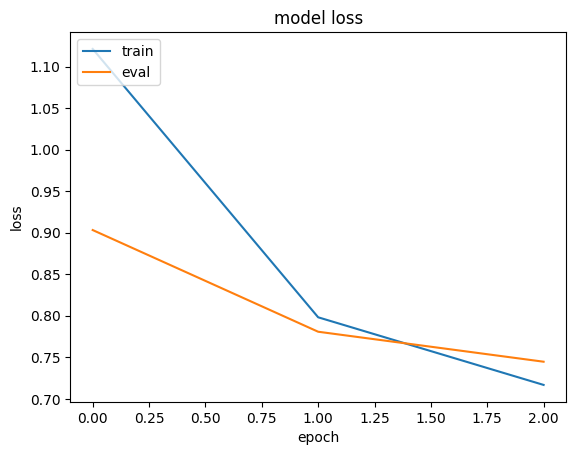
history = run_experiment(baseline_model)

plt.plot(history.history["loss"])
plt.plot(history.history["val_loss"])
plt.title("model loss")
plt.ylabel("loss")
plt.xlabel("epoch")
plt.legend(["train", "eval"], loc="upper left")
plt.show()
Epoch 1/3
   6629/Unknown  17s 3ms/step - loss: 1.4095 - mae: 0.9668

/Library/Frameworks/Python.framework/Versions/3.10/lib/python3.10/contextlib.py:153: UserWarning: Your input ran out of data; interrupting training. Make sure that your dataset or generator can generate at least `steps_per_epoch * epochs` batches. You may need to use the `.repeat()` function when building your dataset.
  self.gen.throw(typ, value, traceback)

 6646/6646 ━━━━━━━━━━━━━━━━━━━━ 18s 3ms/step - loss: 1.4087 - mae: 0.9665 - val_loss: 0.9032 - val_mae: 0.7438
Epoch 2/3
 6646/6646 ━━━━━━━━━━━━━━━━━━━━ 17s 3ms/step - loss: 0.8296 - mae: 0.7193 - val_loss: 0.7807 - val_mae: 0.6976
Epoch 3/3
 6646/6646 ━━━━━━━━━━━━━━━━━━━━ 17s 3ms/step - loss: 0.7305 - mae: 0.6744 - val_loss: 0.7446 - val_mae: 0.6808
實驗 2:節省記憶體的模型
實作商數餘數嵌入作為圖層
商數餘數技術的工作原理如下。對於一組詞彙和嵌入大小 embedding_dim,我們不是建立 vocabulary_size X embedding_dim 嵌入表,而是建立兩個 num_buckets X embedding_dim 嵌入表,其中 num_buckets 遠小於 vocabulary_size。給定項目 index 的嵌入是透過以下步驟產生的
- 將
quotient_index計算為index // num_buckets。 - 將
remainder_index計算為index % num_buckets。 - 使用
quotient_index從第一個嵌入表中查閱quotient_embedding。 - 使用
remainder_index從第二個嵌入表中查閱remainder_embedding。 - 傳回
quotient_embedding*remainder_embedding。
此技術不僅減少了需要儲存和訓練的嵌入向量數量,還為大小為 embedding_dim 的每個項目產生唯一的嵌入向量。請注意,q_embedding 和 r_embedding 可以使用其他運算(例如 Add 和 Concatenate)組合。
class QREmbedding(keras.layers.Layer):
    def __init__(self, vocabulary, embedding_dim, num_buckets, name=None):
        super().__init__(name=name)
        self.num_buckets = num_buckets

        self.index_lookup = StringLookup(
            vocabulary=vocabulary, mask_token=None, num_oov_indices=0
        )
        self.q_embeddings = layers.Embedding(
            num_buckets,
            embedding_dim,
        )
        self.r_embeddings = layers.Embedding(
            num_buckets,
            embedding_dim,
        )

    def call(self, inputs):
        # Get the item index.
        embedding_index = self.index_lookup(inputs)
        # Get the quotient index.
        quotient_index = tf.math.floordiv(embedding_index, self.num_buckets)
        # Get the reminder index.
        remainder_index = tf.math.floormod(embedding_index, self.num_buckets)
        # Lookup the quotient_embedding using the quotient_index.
        quotient_embedding = self.q_embeddings(quotient_index)
        # Lookup the remainder_embedding using the remainder_index.
        remainder_embedding = self.r_embeddings(remainder_index)
        # Use multiplication as a combiner operation
        return quotient_embedding * remainder_embedding
實作混合維度嵌入作為圖層
在混合維度嵌入技術中,我們為經常查詢的項目訓練具有完整維度的嵌入向量,同時為較不頻繁的項目訓練具有縮減維度的嵌入向量,以及一個投影權重矩陣,將低維度嵌入帶到完整的維度。
更精確地說,我們定義了頻率相似的項目區塊。對於每個區塊,都會建立一個 block_vocab_size X block_embedding_dim 嵌入表和 block_embedding_dim X full_embedding_dim 投影權重矩陣。請注意,如果 block_embedding_dim 等於 full_embedding_dim,則投影權重矩陣將變為單位矩陣。給定批次的項目 indices 的嵌入是透過以下步驟產生的
- 對於每個區塊,使用
indices查閱block_embedding_dim嵌入向量,並將其投影到full_embedding_dim。 - 如果項目索引不屬於給定的區塊,則傳回詞彙外嵌入。每個區塊將傳回一個
batch_size X full_embedding_dim張量。 - 會將遮罩套用到從每個區塊傳回的嵌入,以便將詞彙外嵌入轉換為零向量。也就是說,對於批次中的每個項目,會從所有區塊嵌入中傳回單個非零嵌入向量。
- 從區塊中擷取的嵌入會使用總和組合,以產生最終的
batch_size X full_embedding_dim張量。
class MDEmbedding(keras.layers.Layer):
    def __init__(
        self, blocks_vocabulary, blocks_embedding_dims, base_embedding_dim, name=None
    ):
        super().__init__(name=name)
        self.num_blocks = len(blocks_vocabulary)

        # Create vocab to block lookup.
        keys = []
        values = []
        for block_idx, block_vocab in enumerate(blocks_vocabulary):
            keys.extend(block_vocab)
            values.extend([block_idx] * len(block_vocab))
        self.vocab_to_block = tf.lookup.StaticHashTable(
            tf.lookup.KeyValueTensorInitializer(keys, values), default_value=-1
        )

        self.block_embedding_encoders = []
        self.block_embedding_projectors = []

        # Create block embedding encoders and projectors.
        for idx in range(self.num_blocks):
            vocabulary = blocks_vocabulary[idx]
            embedding_dim = blocks_embedding_dims[idx]
            block_embedding_encoder = embedding_encoder(
                vocabulary, embedding_dim, num_oov_indices=1
            )
            self.block_embedding_encoders.append(block_embedding_encoder)
            if embedding_dim == base_embedding_dim:
                self.block_embedding_projectors.append(layers.Lambda(lambda x: x))
            else:
                self.block_embedding_projectors.append(
                    layers.Dense(units=base_embedding_dim)
                )

    def call(self, inputs):
        # Get block index for each input item.
        block_indicies = self.vocab_to_block.lookup(inputs)
        # Initialize output embeddings to zeros.
        embeddings = tf.zeros(shape=(tf.shape(inputs)[0], base_embedding_dim))
        # Generate embeddings from blocks.
        for idx in range(self.num_blocks):
            # Lookup embeddings from the current block.
            block_embeddings = self.block_embedding_encoders[idx](inputs)
            # Project embeddings to base_embedding_dim.
            block_embeddings = self.block_embedding_projectors[idx](block_embeddings)
            # Create a mask to filter out embeddings of items that do not belong to the current block.
            mask = tf.expand_dims(tf.cast(block_indicies == idx, tf.dtypes.float32), 1)
            # Set the embeddings for the items not belonging to the current block to zeros.
            block_embeddings = block_embeddings * mask
            # Add the block embeddings to the final embeddings.
            embeddings += block_embeddings

        return embeddings
實作節省記憶體的模型
在此實驗中,我們將使用商數餘數技術來減少使用者嵌入的大小,並使用混合維度技術來減少電影嵌入的大小。
雖然在 論文中,使用 alpha-power 規則來決定每個區塊的嵌入維度,但我們只是根據電影受歡迎程度的長條圖視覺化,設定區塊的數量和每個區塊的嵌入維度。
movie_frequencies = ratings_data["movie_id"].value_counts()
movie_frequencies.hist(bins=10)
<Axes: >
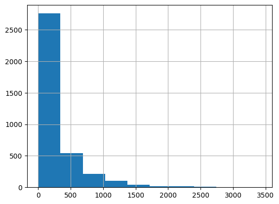
您可以看到我們可以將電影分組為三個區塊,並分別為它們分配 64、32 和 16 個嵌入維度。請隨意試驗不同的區塊數量和維度。
sorted_movie_vocabulary = list(movie_frequencies.keys())

movie_blocks_vocabulary = [
    sorted_movie_vocabulary[:400],  # high popularity movies block
    sorted_movie_vocabulary[400:1700],  # normal popularity movies block
    sorted_movie_vocabulary[1700:],  # low popularity movies block
]

movie_blocks_embedding_dims = [64, 32, 16]

user_embedding_num_buckets = len(user_vocabulary) // 50


def create_memory_efficient_model():
    # Take the user as an input.
    user_input = layers.Input(name="user_id", shape=(), dtype="string")
    # Get user embedding.
    user_embedding = QREmbedding(
        vocabulary=user_vocabulary,
        embedding_dim=base_embedding_dim,
        num_buckets=user_embedding_num_buckets,
        name="user_embedding",
    )(user_input)

    # Take the movie as an input.
    movie_input = layers.Input(name="movie_id", shape=(), dtype="string")
    # Get embedding.
    movie_embedding = MDEmbedding(
        blocks_vocabulary=movie_blocks_vocabulary,
        blocks_embedding_dims=movie_blocks_embedding_dims,
        base_embedding_dim=base_embedding_dim,
        name="movie_embedding",
    )(movie_input)

    # Compute dot product similarity between user and movie embeddings.
    logits = layers.Dot(axes=1, name="dot_similarity")(
        [user_embedding, movie_embedding]
    )
    # Convert to rating scale.
    prediction = keras.activations.sigmoid(logits) * 5
    # Create the model.
    model = keras.Model(
        inputs=[user_input, movie_input], outputs=prediction, name="baseline_model"
    )
    return model


memory_efficient_model = create_memory_efficient_model()
memory_efficient_model.summary()
/Users/fchollet/Library/Python/3.10/lib/python/site-packages/numpy/core/numeric.py:2468: FutureWarning: elementwise comparison failed; returning scalar instead, but in the future will perform elementwise comparison
  return bool(asarray(a1 == a2).all())
Model: "baseline_model"
┏━━━━━━━━━━━━━━━━━━━━━┳━━━━━━━━━━━━━━━━━━━┳━━━━━━━━━┳━━━━━━━━━━━━━━━━━━━━━━┓
┃ Layer (type)        ┃ Output Shape      ┃ Param # ┃ Connected to         ┃
┡━━━━━━━━━━━━━━━━━━━━━╇━━━━━━━━━━━━━━━━━━━╇━━━━━━━━━╇━━━━━━━━━━━━━━━━━━━━━━┩
│ user_id             │ (None)            │       0 │ -                    │
│ (InputLayer)        │                   │         │                      │
├─────────────────────┼───────────────────┼─────────┼──────────────────────┤
│ movie_id            │ (None)            │       0 │ -                    │
│ (InputLayer)        │                   │         │                      │
├─────────────────────┼───────────────────┼─────────┼──────────────────────┤
│ user_embedding      │ (None, 64)        │  15,360 │ user_id[0][0]        │
│ (QREmbedding)       │                   │         │                      │
├─────────────────────┼───────────────────┼─────────┼──────────────────────┤
│ movie_embedding     │ (None, 64)        │ 102,608 │ movie_id[0][0]       │
│ (MDEmbedding)       │                   │         │                      │
├─────────────────────┼───────────────────┼─────────┼──────────────────────┤
│ dot_similarity      │ (None, 1)         │       0 │ user_embedding[0][0… │
│ (Dot)               │                   │         │ movie_embedding[0][… │
├─────────────────────┼───────────────────┼─────────┼──────────────────────┤
│ sigmoid_1 (Sigmoid) │ (None, 1)         │       0 │ dot_similarity[0][0] │
├─────────────────────┼───────────────────┼─────────┼──────────────────────┤
│ multiply_1          │ (None, 1)         │       0 │ sigmoid_1[0][0]      │
│ (Multiply)          │                   │         │                      │
└─────────────────────┴───────────────────┴─────────┴──────────────────────┘
Total params: 117,968 (460.81 KB)
Trainable params: 117,968 (460.81 KB)
Non-trainable params: 0 (0.00 B)
請注意,可訓練參數的數量為 117,968,這比基準模型中的參數數量少 5 倍以上。
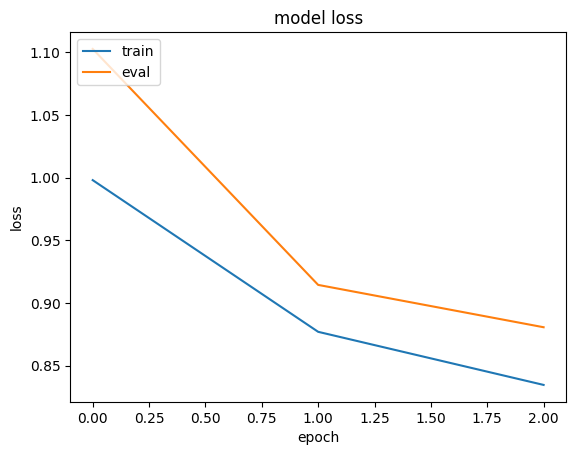
history = run_experiment(memory_efficient_model)

plt.plot(history.history["loss"])
plt.plot(history.history["val_loss"])
plt.title("model loss")
plt.ylabel("loss")
plt.xlabel("epoch")
plt.legend(["train", "eval"], loc="upper left")
plt.show()
Epoch 1/3
   6622/Unknown  6s 891us/step - loss: 1.1938 - mae: 0.8780

/Library/Frameworks/Python.framework/Versions/3.10/lib/python3.10/contextlib.py:153: UserWarning: Your input ran out of data; interrupting training. Make sure that your dataset or generator can generate at least `steps_per_epoch * epochs` batches. You may need to use the `.repeat()` function when building your dataset.
  self.gen.throw(typ, value, traceback)

 6646/6646 ━━━━━━━━━━━━━━━━━━━━ 7s 992us/step - loss: 1.1931 - mae: 0.8777 - val_loss: 1.1027 - val_mae: 0.8179
Epoch 2/3
 6646/6646 ━━━━━━━━━━━━━━━━━━━━ 7s 1ms/step - loss: 0.8908 - mae: 0.7488 - val_loss: 0.9144 - val_mae: 0.7549
Epoch 3/3
 6646/6646 ━━━━━━━━━━━━━━━━━━━━ 7s 980us/step - loss: 0.8419 - mae: 0.7278 - val_loss: 0.8806 - val_mae: 0.7419