估算模型訓練所需的樣本大小
作者: JacoVerster
建立日期 2021/05/20
上次修改日期 2021/06/06
說明: 建立訓練集大小與模型準確度之間關係的模型。

簡介
在許多現實情境中,可用於訓練深度學習模型的圖像資料量有限。在醫學影像領域尤其如此,因為資料集建立成本高昂。當處理新的問題時,通常會出現的第一個問題是:「我們需要多少張圖像才能訓練出足夠好的機器學習模型?」
在大多數情況下,一小組樣本是可用的,我們可以使用它來建立訓練資料大小和模型效能之間的關係模型。此模型可用於估算達到所需模型效能所需的最佳影像數量。
Balki 等人對樣本大小決定方法進行了系統性綜述,其中提供了數種樣本大小決定方法的範例。在本範例中,使用平衡的子取樣方案來決定模型的最佳樣本大小。方法是選擇一個由 Y 個影像組成的隨機子樣本,並使用此子樣本來訓練模型。然後在獨立的測試集上評估模型。對於每個子樣本,此過程重複 N 次,並進行替換,以允許建構觀察到的效能的平均值和信賴區間。
設定
import os

os.environ["KERAS_BACKEND"] = "tensorflow"

import matplotlib.pyplot as plt
import numpy as np
import tensorflow as tf
import keras
from keras import layers
import tensorflow_datasets as tfds

# Define seed and fixed variables
seed = 42
keras.utils.set_random_seed(seed)
AUTO = tf.data.AUTOTUNE
載入 TensorFlow 資料集並轉換為 NumPy 陣列
我們將使用 TF Flowers 資料集。
# Specify dataset parameters
dataset_name = "tf_flowers"
batch_size = 64
image_size = (224, 224)

# Load data from tfds and split 10% off for a test set
(train_data, test_data), ds_info = tfds.load(
    dataset_name,
    split=["train[:90%]", "train[90%:]"],
    shuffle_files=True,
    as_supervised=True,
    with_info=True,
)

# Extract number of classes and list of class names
num_classes = ds_info.features["label"].num_classes
class_names = ds_info.features["label"].names

print(f"Number of classes: {num_classes}")
print(f"Class names: {class_names}")


# Convert datasets to NumPy arrays
def dataset_to_array(dataset, image_size, num_classes):
    images, labels = [], []
    for img, lab in dataset.as_numpy_iterator():
        images.append(tf.image.resize(img, image_size).numpy())
        labels.append(tf.one_hot(lab, num_classes))
    return np.array(images), np.array(labels)


img_train, label_train = dataset_to_array(train_data, image_size, num_classes)
img_test, label_test = dataset_to_array(test_data, image_size, num_classes)

num_train_samples = len(img_train)
print(f"Number of training samples: {num_train_samples}")
Number of classes: 5
Class names: ['dandelion', 'daisy', 'tulips', 'sunflowers', 'roses']
Number of training samples: 3303
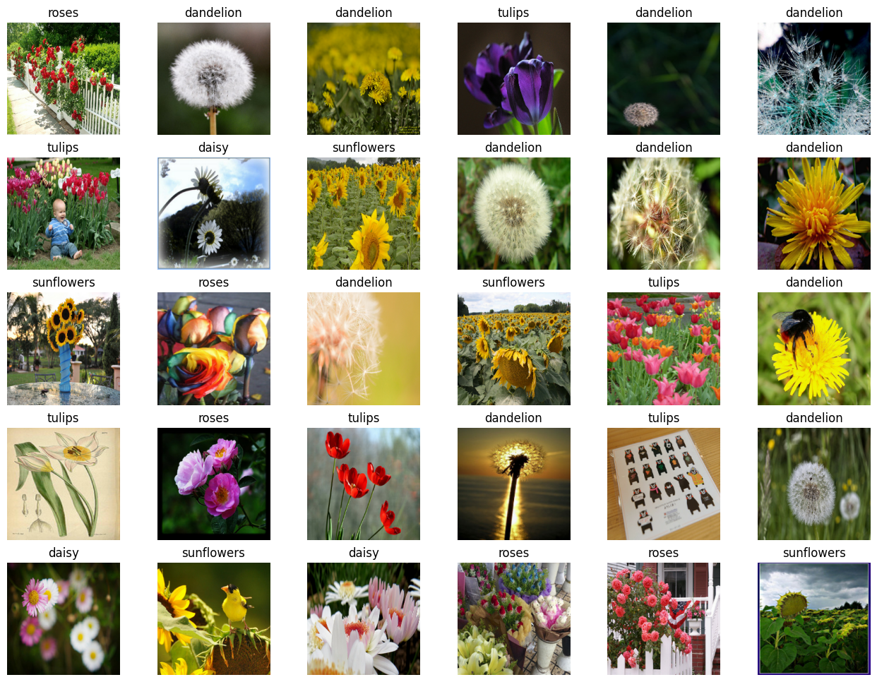
繪製測試集中的幾個範例
plt.figure(figsize=(16, 12))
for n in range(30):
    ax = plt.subplot(5, 6, n + 1)
    plt.imshow(img_test[n].astype("uint8"))
    plt.title(np.array(class_names)[label_test[n] == True][0])
    plt.axis("off")
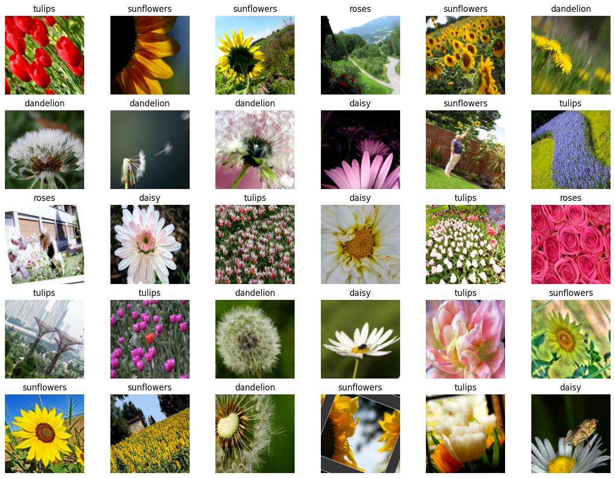
增強
使用 keras 預處理層定義影像增強,並將其應用於訓練集。
# Define image augmentation model
image_augmentation = keras.Sequential(
    [
        layers.RandomFlip(mode="horizontal"),
        layers.RandomRotation(factor=0.1),
        layers.RandomZoom(height_factor=(-0.1, -0)),
        layers.RandomContrast(factor=0.1),
    ],
)

# Apply the augmentations to the training images and plot a few examples
img_train = image_augmentation(img_train).numpy()

plt.figure(figsize=(16, 12))
for n in range(30):
    ax = plt.subplot(5, 6, n + 1)
    plt.imshow(img_train[n].astype("uint8"))
    plt.title(np.array(class_names)[label_train[n] == True][0])
    plt.axis("off")
定義模型建置與訓練函數
我們建立一些便利函數,以建置轉移學習模型、編譯並訓練模型,以及解除凍結層進行微調。
def build_model(num_classes, img_size=image_size[0], top_dropout=0.3):
    """Creates a classifier based on pre-trained MobileNetV2.

    Arguments:
        num_classes: Int, number of classese to use in the softmax layer.
        img_size: Int, square size of input images (defaults is 224).
        top_dropout: Int, value for dropout layer (defaults is 0.3).

    Returns:
        Uncompiled Keras model.
    """

    # Create input and pre-processing layers for MobileNetV2
    inputs = layers.Input(shape=(img_size, img_size, 3))
    x = layers.Rescaling(scale=1.0 / 127.5, offset=-1)(inputs)
    model = keras.applications.MobileNetV2(
        include_top=False, weights="imagenet", input_tensor=x
    )

    # Freeze the pretrained weights
    model.trainable = False

    # Rebuild top
    x = layers.GlobalAveragePooling2D(name="avg_pool")(model.output)
    x = layers.Dropout(top_dropout)(x)
    outputs = layers.Dense(num_classes, activation="softmax")(x)
    model = keras.Model(inputs, outputs)

    print("Trainable weights:", len(model.trainable_weights))
    print("Non_trainable weights:", len(model.non_trainable_weights))
    return model


def compile_and_train(
    model,
    training_data,
    training_labels,
    metrics=[keras.metrics.AUC(name="auc"), "acc"],
    optimizer=keras.optimizers.Adam(),
    patience=5,
    epochs=5,
):
    """Compiles and trains the model.

    Arguments:
        model: Uncompiled Keras model.
        training_data: NumPy Array, training data.
        training_labels: NumPy Array, training labels.
        metrics: Keras/TF metrics, requires at least 'auc' metric (default is
                `[keras.metrics.AUC(name='auc'), 'acc']`).
        optimizer: Keras/TF optimizer (defaults is `keras.optimizers.Adam()).
        patience: Int, epochsfor EarlyStopping patience (defaults is 5).
        epochs: Int, number of epochs to train (default is 5).

    Returns:
        Training history for trained Keras model.
    """

    stopper = keras.callbacks.EarlyStopping(
        monitor="val_auc",
        mode="max",
        min_delta=0,
        patience=patience,
        verbose=1,
        restore_best_weights=True,
    )

    model.compile(loss="categorical_crossentropy", optimizer=optimizer, metrics=metrics)

    history = model.fit(
        x=training_data,
        y=training_labels,
        batch_size=batch_size,
        epochs=epochs,
        validation_split=0.1,
        callbacks=[stopper],
    )
    return history


def unfreeze(model, block_name, verbose=0):
    """Unfreezes Keras model layers.

    Arguments:
        model: Keras model.
        block_name: Str, layer name for example block_name = 'block4'.
                    Checks if supplied string is in the layer name.
        verbose: Int, 0 means silent, 1 prints out layers trainability status.

    Returns:
        Keras model with all layers after (and including) the specified
        block_name to trainable, excluding BatchNormalization layers.
    """

    # Unfreeze from block_name onwards
    set_trainable = False

    for layer in model.layers:
        if block_name in layer.name:
            set_trainable = True
        if set_trainable and not isinstance(layer, layers.BatchNormalization):
            layer.trainable = True
            if verbose == 1:
                print(layer.name, "trainable")
        else:
            if verbose == 1:
                print(layer.name, "NOT trainable")
    print("Trainable weights:", len(model.trainable_weights))
    print("Non-trainable weights:", len(model.non_trainable_weights))
    return model
定義迭代訓練函數
為了在多個子樣本集上訓練模型,我們需要建立迭代訓練函數。
def train_model(training_data, training_labels):
    """Trains the model as follows:

    - Trains only the top layers for 10 epochs.
    - Unfreezes deeper layers.
    - Train for 20 more epochs.

    Arguments:
        training_data: NumPy Array, training data.
        training_labels: NumPy Array, training labels.

    Returns:
        Model accuracy.
    """

    model = build_model(num_classes)

    # Compile and train top layers
    history = compile_and_train(
        model,
        training_data,
        training_labels,
        metrics=[keras.metrics.AUC(name="auc"), "acc"],
        optimizer=keras.optimizers.Adam(),
        patience=3,
        epochs=10,
    )

    # Unfreeze model from block 10 onwards
    model = unfreeze(model, "block_10")

    # Compile and train for 20 epochs with a lower learning rate
    fine_tune_epochs = 20
    total_epochs = history.epoch[-1] + fine_tune_epochs

    history_fine = compile_and_train(
        model,
        training_data,
        training_labels,
        metrics=[keras.metrics.AUC(name="auc"), "acc"],
        optimizer=keras.optimizers.Adam(learning_rate=1e-4),
        patience=5,
        epochs=total_epochs,
    )

    # Calculate model accuracy on the test set
    _, _, acc = model.evaluate(img_test, label_test)
    return np.round(acc, 4)
迭代訓練模型
現在我們有了模型建置函數和支援迭代函數,我們可以在多個子樣本分割上訓練模型。
- 我們選擇子樣本分割為下載資料集的 5%、10%、25% 和 50%。我們假設目前只有 50% 的實際資料可用。
- 我們在每個分割處從頭開始訓練模型 5 次,並記錄準確度值。
請注意,這會訓練 20 個模型,需要一些時間。請確保您的 GPU 執行階段為啟動狀態。
為了使此範例更輕量,將提供先前訓練執行中的樣本資料。
def train_iteratively(sample_splits=[0.05, 0.1, 0.25, 0.5], iter_per_split=5):
    """Trains a model iteratively over several sample splits.

    Arguments:
        sample_splits: List/NumPy array, contains fractions of the trainins set
                        to train over.
        iter_per_split: Int, number of times to train a model per sample split.

    Returns:
        Training accuracy for all splits and iterations and the number of samples
        used for training at each split.
    """
    # Train all the sample models and calculate accuracy
    train_acc = []
    sample_sizes = []

    for fraction in sample_splits:
        print(f"Fraction split: {fraction}")
        # Repeat training 3 times for each sample size
        sample_accuracy = []
        num_samples = int(num_train_samples * fraction)
        for i in range(iter_per_split):
            print(f"Run {i+1} out of {iter_per_split}:")
            # Create fractional subsets
            rand_idx = np.random.randint(num_train_samples, size=num_samples)
            train_img_subset = img_train[rand_idx, :]
            train_label_subset = label_train[rand_idx, :]
            # Train model and calculate accuracy
            accuracy = train_model(train_img_subset, train_label_subset)
            print(f"Accuracy: {accuracy}")
            sample_accuracy.append(accuracy)
        train_acc.append(sample_accuracy)
        sample_sizes.append(num_samples)
    return train_acc, sample_sizes


# Running the above function produces the following outputs
train_acc = [
    [0.8202, 0.7466, 0.8011, 0.8447, 0.8229],
    [0.861, 0.8774, 0.8501, 0.8937, 0.891],
    [0.891, 0.9237, 0.8856, 0.9101, 0.891],
    [0.8937, 0.9373, 0.9128, 0.8719, 0.9128],
]

sample_sizes = [165, 330, 825, 1651]
學習曲線
現在,我們透過在平均準確度點上擬合指數曲線來繪製學習曲線。我們使用 TF 來將指數函數擬合到資料中。
然後,我們將學習曲線外推,以預測在整個訓練集上訓練的模型準確度。
def fit_and_predict(train_acc, sample_sizes, pred_sample_size):
    """Fits a learning curve to model training accuracy results.

    Arguments:
        train_acc: List/Numpy Array, training accuracy for all model
                    training splits and iterations.
        sample_sizes: List/Numpy array, number of samples used for training at
                    each split.
        pred_sample_size: Int, sample size to predict model accuracy based on
                        fitted learning curve.
    """
    x = sample_sizes
    mean_acc = tf.convert_to_tensor([np.mean(i) for i in train_acc])
    error = [np.std(i) for i in train_acc]

    # Define mean squared error cost and exponential curve fit functions
    mse = keras.losses.MeanSquaredError()

    def exp_func(x, a, b):
        return a * x**b

    # Define variables, learning rate and number of epochs for fitting with TF
    a = tf.Variable(0.0)
    b = tf.Variable(0.0)
    learning_rate = 0.01
    training_epochs = 5000

    # Fit the exponential function to the data
    for epoch in range(training_epochs):
        with tf.GradientTape() as tape:
            y_pred = exp_func(x, a, b)
            cost_function = mse(y_pred, mean_acc)
        # Get gradients and compute adjusted weights
        gradients = tape.gradient(cost_function, [a, b])
        a.assign_sub(gradients[0] * learning_rate)
        b.assign_sub(gradients[1] * learning_rate)
    print(f"Curve fit weights: a = {a.numpy()} and b = {b.numpy()}.")

    # We can now estimate the accuracy for pred_sample_size
    max_acc = exp_func(pred_sample_size, a, b).numpy()

    # Print predicted x value and append to plot values
    print(f"A model accuracy of {max_acc} is predicted for {pred_sample_size} samples.")
    x_cont = np.linspace(x[0], pred_sample_size, 100)

    # Build the plot
    fig, ax = plt.subplots(figsize=(12, 6))
    ax.errorbar(x, mean_acc, yerr=error, fmt="o", label="Mean acc & std dev.")
    ax.plot(x_cont, exp_func(x_cont, a, b), "r-", label="Fitted exponential curve.")
    ax.set_ylabel("Model classification accuracy.", fontsize=12)
    ax.set_xlabel("Training sample size.", fontsize=12)
    ax.set_xticks(np.append(x, pred_sample_size))
    ax.set_yticks(np.append(mean_acc, max_acc))
    ax.set_xticklabels(list(np.append(x, pred_sample_size)), rotation=90, fontsize=10)
    ax.yaxis.set_tick_params(labelsize=10)
    ax.set_title("Learning curve: model accuracy vs sample size.", fontsize=14)
    ax.legend(loc=(0.75, 0.75), fontsize=10)
    ax.xaxis.grid(True)
    ax.yaxis.grid(True)
    plt.tight_layout()
    plt.show()

    # The mean absolute error (MAE) is calculated for curve fit to see how well
    # it fits the data. The lower the error the better the fit.
    mae = keras.losses.MeanAbsoluteError()
    print(f"The mae for the curve fit is {mae(mean_acc, exp_func(x, a, b)).numpy()}.")


# We use the whole training set to predict the model accuracy
fit_and_predict(train_acc, sample_sizes, pred_sample_size=num_train_samples)
Curve fit weights: a = 0.6445642113685608 and b = 0.048097413033246994.
A model accuracy of 0.9517362117767334 is predicted for 3303 samples.
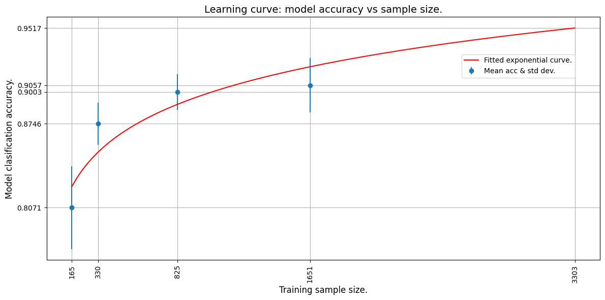
The mae for the curve fit is 0.016098767518997192.
從外推曲線中,我們可以看到 3303 個影像將產生約 95% 的估計準確度。
現在,讓我們使用所有資料(3303 個影像)來訓練模型,看看我們的預測是否準確!
# Now train the model with full dataset to get the actual accuracy
accuracy = train_model(img_train, label_train)
print(f"A model accuracy of {accuracy} is reached on {num_train_samples} images!")
/var/folders/8n/8w8cqnvj01xd4ghznl11nyn000_93_/T/ipykernel_30919/1838736464.py:16: UserWarning: `input_shape` is undefined or non-square, or `rows` is not in [96, 128, 160, 192, 224]. Weights for input shape (224, 224) will be loaded as the default.
  model = keras.applications.MobileNetV2(

Trainable weights: 2
Non_trainable weights: 260
Epoch 1/10
 47/47 ━━━━━━━━━━━━━━━━━━━━ 18s 338ms/step - acc: 0.4305 - auc: 0.7221 - loss: 1.4585 - val_acc: 0.8218 - val_auc: 0.9700 - val_loss: 0.5043
Epoch 2/10
 47/47 ━━━━━━━━━━━━━━━━━━━━ 15s 326ms/step - acc: 0.7666 - auc: 0.9504 - loss: 0.6287 - val_acc: 0.8792 - val_auc: 0.9838 - val_loss: 0.3733
Epoch 3/10
 47/47 ━━━━━━━━━━━━━━━━━━━━ 16s 332ms/step - acc: 0.8252 - auc: 0.9673 - loss: 0.5039 - val_acc: 0.8852 - val_auc: 0.9880 - val_loss: 0.3182
Epoch 4/10
 47/47 ━━━━━━━━━━━━━━━━━━━━ 16s 348ms/step - acc: 0.8458 - auc: 0.9768 - loss: 0.4264 - val_acc: 0.8822 - val_auc: 0.9893 - val_loss: 0.2956
Epoch 5/10
 47/47 ━━━━━━━━━━━━━━━━━━━━ 16s 350ms/step - acc: 0.8661 - auc: 0.9812 - loss: 0.3821 - val_acc: 0.8912 - val_auc: 0.9903 - val_loss: 0.2755
Epoch 6/10
 47/47 ━━━━━━━━━━━━━━━━━━━━ 16s 336ms/step - acc: 0.8656 - auc: 0.9836 - loss: 0.3555 - val_acc: 0.9003 - val_auc: 0.9906 - val_loss: 0.2701
Epoch 7/10
 47/47 ━━━━━━━━━━━━━━━━━━━━ 16s 331ms/step - acc: 0.8800 - auc: 0.9846 - loss: 0.3430 - val_acc: 0.8943 - val_auc: 0.9914 - val_loss: 0.2548
Epoch 8/10
 47/47 ━━━━━━━━━━━━━━━━━━━━ 16s 333ms/step - acc: 0.8917 - auc: 0.9871 - loss: 0.3143 - val_acc: 0.8973 - val_auc: 0.9917 - val_loss: 0.2494
Epoch 9/10
 47/47 ━━━━━━━━━━━━━━━━━━━━ 15s 320ms/step - acc: 0.9003 - auc: 0.9891 - loss: 0.2906 - val_acc: 0.9063 - val_auc: 0.9908 - val_loss: 0.2463
Epoch 10/10
 47/47 ━━━━━━━━━━━━━━━━━━━━ 15s 324ms/step - acc: 0.8997 - auc: 0.9895 - loss: 0.2839 - val_acc: 0.9124 - val_auc: 0.9912 - val_loss: 0.2394
Trainable weights: 24
Non-trainable weights: 238
Epoch 1/29
 47/47 ━━━━━━━━━━━━━━━━━━━━ 27s 537ms/step - acc: 0.8457 - auc: 0.9747 - loss: 0.4365 - val_acc: 0.9094 - val_auc: 0.9916 - val_loss: 0.2692
Epoch 2/29
 47/47 ━━━━━━━━━━━━━━━━━━━━ 24s 502ms/step - acc: 0.9223 - auc: 0.9932 - loss: 0.2198 - val_acc: 0.9033 - val_auc: 0.9891 - val_loss: 0.2826
Epoch 3/29
 47/47 ━━━━━━━━━━━━━━━━━━━━ 25s 534ms/step - acc: 0.9499 - auc: 0.9972 - loss: 0.1399 - val_acc: 0.9003 - val_auc: 0.9910 - val_loss: 0.2804
Epoch 4/29
 47/47 ━━━━━━━━━━━━━━━━━━━━ 26s 554ms/step - acc: 0.9590 - auc: 0.9983 - loss: 0.1130 - val_acc: 0.9396 - val_auc: 0.9968 - val_loss: 0.1510
Epoch 5/29
 47/47 ━━━━━━━━━━━━━━━━━━━━ 25s 533ms/step - acc: 0.9805 - auc: 0.9996 - loss: 0.0538 - val_acc: 0.9486 - val_auc: 0.9914 - val_loss: 0.1795
Epoch 6/29
 47/47 ━━━━━━━━━━━━━━━━━━━━ 24s 516ms/step - acc: 0.9949 - auc: 1.0000 - loss: 0.0226 - val_acc: 0.9124 - val_auc: 0.9833 - val_loss: 0.3186
Epoch 7/29
 47/47 ━━━━━━━━━━━━━━━━━━━━ 25s 534ms/step - acc: 0.9900 - auc: 0.9999 - loss: 0.0297 - val_acc: 0.9275 - val_auc: 0.9881 - val_loss: 0.3017
Epoch 8/29
 47/47 ━━━━━━━━━━━━━━━━━━━━ 25s 536ms/step - acc: 0.9910 - auc: 0.9999 - loss: 0.0228 - val_acc: 0.9426 - val_auc: 0.9927 - val_loss: 0.1938
Epoch 9/29
 47/47 ━━━━━━━━━━━━━━━━━━━━ 0s 489ms/step - acc: 0.9995 - auc: 1.0000 - loss: 0.0069Restoring model weights from the end of the best epoch: 4.
 47/47 ━━━━━━━━━━━━━━━━━━━━ 25s 527ms/step - acc: 0.9995 - auc: 1.0000 - loss: 0.0068 - val_acc: 0.9426 - val_auc: 0.9919 - val_loss: 0.2957
Epoch 9: early stopping
 12/12 ━━━━━━━━━━━━━━━━━━━━ 2s 170ms/step - acc: 0.9641 - auc: 0.9972 - loss: 0.1264
A model accuracy of 0.9964 is reached on 3303 images!
結論
我們看到,使用 3303 個影像時,模型準確度約達到 94-96%*。這與我們的估計相當接近!
即使我們只使用了 50% 的資料集(1651 個影像),我們也能建立模型訓練行為的模型,並預測給定數量影像的模型準確度。當可以使用較小的資料集,並且已證明可以在深度學習模型上收斂,但需要更多影像時,可以使用相同的方法來預測達到所需準確度所需的影像數量。影像計數預測可用於規劃和編列預算以進行進一步的影像收集計畫。