使用卷積 LSTM 進行下一幀影片預測
作者: Amogh Joshi
建立日期 2021/06/02
上次修改日期 2023/11/10
描述: 如何建立和訓練用於下一幀影片預測的卷積 LSTM 模型。

簡介
卷積 LSTM 架構透過在 LSTM 層中引入卷積遞迴單元,將時間序列處理和電腦視覺結合在一起。在本範例中,我們將探索卷積 LSTM 模型在下一幀預測中的應用,即預測給定一系列過去幀後,接下來會出現哪些影片幀的過程。
設定
import numpy as np
import matplotlib.pyplot as plt

import keras
from keras import layers

import io
import imageio
from IPython.display import Image, display
from ipywidgets import widgets, Layout, HBox
數據集建構
在本範例中,我們將使用 移動 MNIST 數據集。
我們將下載數據集,然後建構和預處理訓練和驗證集。
對於下一幀預測,我們的模型將使用先前的幀 (我們將其稱為 f_n) 來預測新的幀 (稱為 f_(n + 1))。為了讓模型能夠產生這些預測,我們需要處理數據,使其具有「移動」的輸入和輸出,其中輸入數據是幀 x_n,用於預測幀 y_(n + 1)。
# Download and load the dataset.
fpath = keras.utils.get_file(
    "moving_mnist.npy",
    "http://www.cs.toronto.edu/~nitish/unsupervised_video/mnist_test_seq.npy",
)
dataset = np.load(fpath)

# Swap the axes representing the number of frames and number of data samples.
dataset = np.swapaxes(dataset, 0, 1)
# We'll pick out 1000 of the 10000 total examples and use those.
dataset = dataset[:1000, ...]
# Add a channel dimension since the images are grayscale.
dataset = np.expand_dims(dataset, axis=-1)

# Split into train and validation sets using indexing to optimize memory.
indexes = np.arange(dataset.shape[0])
np.random.shuffle(indexes)
train_index = indexes[: int(0.9 * dataset.shape[0])]
val_index = indexes[int(0.9 * dataset.shape[0]) :]
train_dataset = dataset[train_index]
val_dataset = dataset[val_index]

# Normalize the data to the 0-1 range.
train_dataset = train_dataset / 255
val_dataset = val_dataset / 255


# We'll define a helper function to shift the frames, where
# `x` is frames 0 to n - 1, and `y` is frames 1 to n.
def create_shifted_frames(data):
    x = data[:, 0 : data.shape[1] - 1, :, :]
    y = data[:, 1 : data.shape[1], :, :]
    return x, y


# Apply the processing function to the datasets.
x_train, y_train = create_shifted_frames(train_dataset)
x_val, y_val = create_shifted_frames(val_dataset)

# Inspect the dataset.
print("Training Dataset Shapes: " + str(x_train.shape) + ", " + str(y_train.shape))
print("Validation Dataset Shapes: " + str(x_val.shape) + ", " + str(y_val.shape))
Downloading data from http://www.cs.toronto.edu/~nitish/unsupervised_video/mnist_test_seq.npy
 819200096/819200096 ━━━━━━━━━━━━━━━━━━━━ 116s 0us/step
Training Dataset Shapes: (900, 19, 64, 64, 1), (900, 19, 64, 64, 1)
Validation Dataset Shapes: (100, 19, 64, 64, 1), (100, 19, 64, 64, 1)
數據視覺化
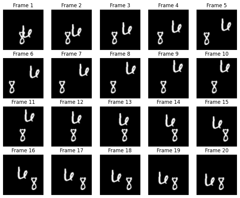
我們的數據包含幀序列,每個幀都用於預測即將到來的幀。讓我們來看看其中一些連續幀。
# Construct a figure on which we will visualize the images.
fig, axes = plt.subplots(4, 5, figsize=(10, 8))

# Plot each of the sequential images for one random data example.
data_choice = np.random.choice(range(len(train_dataset)), size=1)[0]
for idx, ax in enumerate(axes.flat):
    ax.imshow(np.squeeze(train_dataset[data_choice][idx]), cmap="gray")
    ax.set_title(f"Frame {idx + 1}")
    ax.axis("off")

# Print information and display the figure.
print(f"Displaying frames for example {data_choice}.")
plt.show()
Displaying frames for example 95.
模型建構
若要建構卷積 LSTM 模型,我們將使用 ConvLSTM2D 層,它將接受形狀為 (batch_size, num_frames, width, height, channels) 的輸入,並傳回相同形狀的預測影片。
# Construct the input layer with no definite frame size.
inp = layers.Input(shape=(None, *x_train.shape[2:]))

# We will construct 3 `ConvLSTM2D` layers with batch normalization,
# followed by a `Conv3D` layer for the spatiotemporal outputs.
x = layers.ConvLSTM2D(
    filters=64,
    kernel_size=(5, 5),
    padding="same",
    return_sequences=True,
    activation="relu",
)(inp)
x = layers.BatchNormalization()(x)
x = layers.ConvLSTM2D(
    filters=64,
    kernel_size=(3, 3),
    padding="same",
    return_sequences=True,
    activation="relu",
)(x)
x = layers.BatchNormalization()(x)
x = layers.ConvLSTM2D(
    filters=64,
    kernel_size=(1, 1),
    padding="same",
    return_sequences=True,
    activation="relu",
)(x)
x = layers.Conv3D(
    filters=1, kernel_size=(3, 3, 3), activation="sigmoid", padding="same"
)(x)

# Next, we will build the complete model and compile it.
model = keras.models.Model(inp, x)
model.compile(
    loss=keras.losses.binary_crossentropy,
    optimizer=keras.optimizers.Adam(),
)
模型訓練
在建構模型和數據後,我們現在可以訓練模型。
# Define some callbacks to improve training.
early_stopping = keras.callbacks.EarlyStopping(monitor="val_loss", patience=10)
reduce_lr = keras.callbacks.ReduceLROnPlateau(monitor="val_loss", patience=5)

# Define modifiable training hyperparameters.
epochs = 20
batch_size = 5

# Fit the model to the training data.
model.fit(
    x_train,
    y_train,
    batch_size=batch_size,
    epochs=epochs,
    validation_data=(x_val, y_val),
    callbacks=[early_stopping, reduce_lr],
)
Epoch 1/20
 180/180 ━━━━━━━━━━━━━━━━━━━━ 50s 226ms/step - loss: 0.1510 - val_loss: 0.2966 - learning_rate: 0.0010
Epoch 2/20
 180/180 ━━━━━━━━━━━━━━━━━━━━ 40s 219ms/step - loss: 0.0287 - val_loss: 0.1766 - learning_rate: 0.0010
Epoch 3/20
 180/180 ━━━━━━━━━━━━━━━━━━━━ 40s 219ms/step - loss: 0.0269 - val_loss: 0.0661 - learning_rate: 0.0010
Epoch 4/20
 180/180 ━━━━━━━━━━━━━━━━━━━━ 40s 219ms/step - loss: 0.0264 - val_loss: 0.0279 - learning_rate: 0.0010
Epoch 5/20
 180/180 ━━━━━━━━━━━━━━━━━━━━ 40s 219ms/step - loss: 0.0258 - val_loss: 0.0254 - learning_rate: 0.0010
Epoch 6/20
 180/180 ━━━━━━━━━━━━━━━━━━━━ 40s 219ms/step - loss: 0.0256 - val_loss: 0.0253 - learning_rate: 0.0010
Epoch 7/20
 180/180 ━━━━━━━━━━━━━━━━━━━━ 40s 219ms/step - loss: 0.0251 - val_loss: 0.0248 - learning_rate: 0.0010
Epoch 8/20
 180/180 ━━━━━━━━━━━━━━━━━━━━ 40s 219ms/step - loss: 0.0251 - val_loss: 0.0251 - learning_rate: 0.0010
Epoch 9/20
 180/180 ━━━━━━━━━━━━━━━━━━━━ 40s 219ms/step - loss: 0.0247 - val_loss: 0.0243 - learning_rate: 0.0010
Epoch 10/20
 180/180 ━━━━━━━━━━━━━━━━━━━━ 40s 219ms/step - loss: 0.0246 - val_loss: 0.0246 - learning_rate: 0.0010
Epoch 11/20
 180/180 ━━━━━━━━━━━━━━━━━━━━ 40s 219ms/step - loss: 0.0245 - val_loss: 0.0247 - learning_rate: 0.0010
Epoch 12/20
 180/180 ━━━━━━━━━━━━━━━━━━━━ 40s 219ms/step - loss: 0.0241 - val_loss: 0.0243 - learning_rate: 0.0010
Epoch 13/20
 180/180 ━━━━━━━━━━━━━━━━━━━━ 40s 219ms/step - loss: 0.0244 - val_loss: 0.0245 - learning_rate: 0.0010
Epoch 14/20
 180/180 ━━━━━━━━━━━━━━━━━━━━ 40s 219ms/step - loss: 0.0241 - val_loss: 0.0241 - learning_rate: 0.0010
Epoch 15/20
 180/180 ━━━━━━━━━━━━━━━━━━━━ 40s 219ms/step - loss: 0.0243 - val_loss: 0.0241 - learning_rate: 0.0010
Epoch 16/20
 180/180 ━━━━━━━━━━━━━━━━━━━━ 40s 219ms/step - loss: 0.0242 - val_loss: 0.0242 - learning_rate: 0.0010
Epoch 17/20
 180/180 ━━━━━━━━━━━━━━━━━━━━ 40s 219ms/step - loss: 0.0240 - val_loss: 0.0240 - learning_rate: 0.0010
Epoch 18/20
 180/180 ━━━━━━━━━━━━━━━━━━━━ 40s 219ms/step - loss: 0.0240 - val_loss: 0.0243 - learning_rate: 0.0010
Epoch 19/20
 180/180 ━━━━━━━━━━━━━━━━━━━━ 40s 219ms/step - loss: 0.0240 - val_loss: 0.0244 - learning_rate: 0.0010
Epoch 20/20
 180/180 ━━━━━━━━━━━━━━━━━━━━ 40s 219ms/step - loss: 0.0237 - val_loss: 0.0238 - learning_rate: 1.0000e-04

<keras.src.callbacks.history.History at 0x7ff294f9c340>
幀預測視覺化
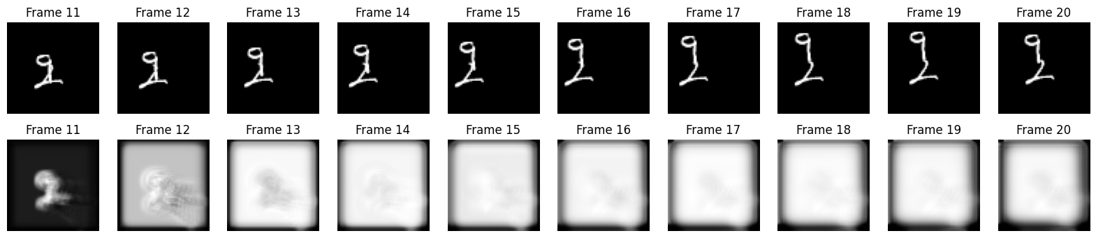
在建構和訓練我們的模型後,我們可以根據新的影片產生一些範例幀預測。
我們將從驗證集中選擇一個隨機範例,然後從中選擇前十個幀。從那裡,我們可以讓模型預測 10 個新幀,我們可以將其與基本事實幀預測進行比較。
# Select a random example from the validation dataset.
example = val_dataset[np.random.choice(range(len(val_dataset)), size=1)[0]]

# Pick the first/last ten frames from the example.
frames = example[:10, ...]
original_frames = example[10:, ...]

# Predict a new set of 10 frames.
for _ in range(10):
    # Extract the model's prediction and post-process it.
    new_prediction = model.predict(np.expand_dims(frames, axis=0))
    new_prediction = np.squeeze(new_prediction, axis=0)
    predicted_frame = np.expand_dims(new_prediction[-1, ...], axis=0)

    # Extend the set of prediction frames.
    frames = np.concatenate((frames, predicted_frame), axis=0)

# Construct a figure for the original and new frames.
fig, axes = plt.subplots(2, 10, figsize=(20, 4))

# Plot the original frames.
for idx, ax in enumerate(axes[0]):
    ax.imshow(np.squeeze(original_frames[idx]), cmap="gray")
    ax.set_title(f"Frame {idx + 11}")
    ax.axis("off")

# Plot the new frames.
new_frames = frames[10:, ...]
for idx, ax in enumerate(axes[1]):
    ax.imshow(np.squeeze(new_frames[idx]), cmap="gray")
    ax.set_title(f"Frame {idx + 11}")
    ax.axis("off")

# Display the figure.
plt.show()
 1/1 ━━━━━━━━━━━━━━━━━━━━ 2s 2s/step
 1/1 ━━━━━━━━━━━━━━━━━━━━ 1s 800ms/step
 1/1 ━━━━━━━━━━━━━━━━━━━━ 1s 805ms/step
 1/1 ━━━━━━━━━━━━━━━━━━━━ 1s 790ms/step
 1/1 ━━━━━━━━━━━━━━━━━━━━ 1s 821ms/step
 1/1 ━━━━━━━━━━━━━━━━━━━━ 1s 824ms/step
 1/1 ━━━━━━━━━━━━━━━━━━━━ 1s 928ms/step
 1/1 ━━━━━━━━━━━━━━━━━━━━ 1s 813ms/step
 1/1 ━━━━━━━━━━━━━━━━━━━━ 1s 810ms/step
 1/1 ━━━━━━━━━━━━━━━━━━━━ 1s 814ms/step
預測影片
最後,我們將從驗證集中選擇幾個範例,並使用它們建構一些 GIF,以查看模型的預測影片。
您可以使用託管在 Hugging Face Hub 上的已訓練模型,並在 Hugging Face Spaces 上嘗試演示。
# Select a few random examples from the dataset.
examples = val_dataset[np.random.choice(range(len(val_dataset)), size=5)]

# Iterate over the examples and predict the frames.
predicted_videos = []
for example in examples:
    # Pick the first/last ten frames from the example.
    frames = example[:10, ...]
    original_frames = example[10:, ...]
    new_predictions = np.zeros(shape=(10, *frames[0].shape))

    # Predict a new set of 10 frames.
    for i in range(10):
        # Extract the model's prediction and post-process it.
        frames = example[: 10 + i + 1, ...]
        new_prediction = model.predict(np.expand_dims(frames, axis=0))
        new_prediction = np.squeeze(new_prediction, axis=0)
        predicted_frame = np.expand_dims(new_prediction[-1, ...], axis=0)

        # Extend the set of prediction frames.
        new_predictions[i] = predicted_frame

    # Create and save GIFs for each of the ground truth/prediction images.
    for frame_set in [original_frames, new_predictions]:
        # Construct a GIF from the selected video frames.
        current_frames = np.squeeze(frame_set)
        current_frames = current_frames[..., np.newaxis] * np.ones(3)
        current_frames = (current_frames * 255).astype(np.uint8)
        current_frames = list(current_frames)

        # Construct a GIF from the frames.
        with io.BytesIO() as gif:
            imageio.mimsave(gif, current_frames, "GIF", duration=200)
            predicted_videos.append(gif.getvalue())

# Display the videos.
print(" Truth\tPrediction")
for i in range(0, len(predicted_videos), 2):
    # Construct and display an `HBox` with the ground truth and prediction.
    box = HBox(
        [
            widgets.Image(value=predicted_videos[i]),
            widgets.Image(value=predicted_videos[i + 1]),
        ]
    )
    display(box)
 1/1 ━━━━━━━━━━━━━━━━━━━━ 0s 6ms/step
 1/1 ━━━━━━━━━━━━━━━━━━━━ 0s 5ms/step
 1/1 ━━━━━━━━━━━━━━━━━━━━ 0s 5ms/step
 1/1 ━━━━━━━━━━━━━━━━━━━━ 0s 5ms/step
 1/1 ━━━━━━━━━━━━━━━━━━━━ 0s 6ms/step
 1/1 ━━━━━━━━━━━━━━━━━━━━ 0s 6ms/step
 1/1 ━━━━━━━━━━━━━━━━━━━━ 0s 8ms/step
 1/1 ━━━━━━━━━━━━━━━━━━━━ 0s 7ms/step
 1/1 ━━━━━━━━━━━━━━━━━━━━ 0s 7ms/step
 1/1 ━━━━━━━━━━━━━━━━━━━━ 1s 790ms/step
 1/1 ━━━━━━━━━━━━━━━━━━━━ 0s 5ms/step
 1/1 ━━━━━━━━━━━━━━━━━━━━ 0s 5ms/step
 1/1 ━━━━━━━━━━━━━━━━━━━━ 0s 5ms/step
 1/1 ━━━━━━━━━━━━━━━━━━━━ 0s 5ms/step
 1/1 ━━━━━━━━━━━━━━━━━━━━ 0s 6ms/step
 1/1 ━━━━━━━━━━━━━━━━━━━━ 0s 6ms/step
 1/1 ━━━━━━━━━━━━━━━━━━━━ 0s 7ms/step
 1/1 ━━━━━━━━━━━━━━━━━━━━ 0s 7ms/step
 1/1 ━━━━━━━━━━━━━━━━━━━━ 0s 8ms/step
 1/1 ━━━━━━━━━━━━━━━━━━━━ 0s 8ms/step
 1/1 ━━━━━━━━━━━━━━━━━━━━ 0s 6ms/step
 1/1 ━━━━━━━━━━━━━━━━━━━━ 0s 6ms/step
 1/1 ━━━━━━━━━━━━━━━━━━━━ 0s 5ms/step
 1/1 ━━━━━━━━━━━━━━━━━━━━ 0s 6ms/step
 1/1 ━━━━━━━━━━━━━━━━━━━━ 0s 6ms/step
 1/1 ━━━━━━━━━━━━━━━━━━━━ 0s 6ms/step
 1/1 ━━━━━━━━━━━━━━━━━━━━ 0s 7ms/step
 1/1 ━━━━━━━━━━━━━━━━━━━━ 0s 7ms/step
 1/1 ━━━━━━━━━━━━━━━━━━━━ 0s 7ms/step
 1/1 ━━━━━━━━━━━━━━━━━━━━ 0s 8ms/step
 1/1 ━━━━━━━━━━━━━━━━━━━━ 0s 6ms/step
 1/1 ━━━━━━━━━━━━━━━━━━━━ 0s 5ms/step
 1/1 ━━━━━━━━━━━━━━━━━━━━ 0s 6ms/step
 1/1 ━━━━━━━━━━━━━━━━━━━━ 0s 6ms/step
 1/1 ━━━━━━━━━━━━━━━━━━━━ 0s 7ms/step
 1/1 ━━━━━━━━━━━━━━━━━━━━ 0s 8ms/step
 1/1 ━━━━━━━━━━━━━━━━━━━━ 0s 6ms/step
 1/1 ━━━━━━━━━━━━━━━━━━━━ 0s 7ms/step
 1/1 ━━━━━━━━━━━━━━━━━━━━ 0s 7ms/step
 1/1 ━━━━━━━━━━━━━━━━━━━━ 0s 9ms/step
 1/1 ━━━━━━━━━━━━━━━━━━━━ 0s 5ms/step
 1/1 ━━━━━━━━━━━━━━━━━━━━ 0s 5ms/step
 1/1 ━━━━━━━━━━━━━━━━━━━━ 0s 5ms/step
 1/1 ━━━━━━━━━━━━━━━━━━━━ 0s 5ms/step
 1/1 ━━━━━━━━━━━━━━━━━━━━ 0s 6ms/step
 1/1 ━━━━━━━━━━━━━━━━━━━━ 0s 6ms/step
 1/1 ━━━━━━━━━━━━━━━━━━━━ 0s 6ms/step
 1/1 ━━━━━━━━━━━━━━━━━━━━ 0s 7ms/step
 1/1 ━━━━━━━━━━━━━━━━━━━━ 0s 8ms/step
 1/1 ━━━━━━━━━━━━━━━━━━━━ 0s 10ms/step
 Truth  Prediction

HBox(children=(Image(value=b'GIF89a@\x00@\x00\x87\x00\x00\xff\xff\xff\xfe\xfe\xfe\xfd\xfd\xfd\xfc\xfc\xfc\xf8\…

HBox(children=(Image(value=b'GIF89a@\x00@\x00\x86\x00\x00\xff\xff\xff\xfd\xfd\xfd\xfc\xfc\xfc\xfb\xfb\xfb\xf4\…

HBox(children=(Image(value=b'GIF89a@\x00@\x00\x86\x00\x00\xff\xff\xff\xfe\xfe\xfe\xfd\xfd\xfd\xfc\xfc\xfc\xfb\…

HBox(children=(Image(value=b'GIF89a@\x00@\x00\x86\x00\x00\xff\xff\xff\xfe\xfe\xfe\xfd\xfd\xfd\xfc\xfc\xfc\xfb\…

HBox(children=(Image(value=b'GIF89a@\x00@\x00\x86\x00\x00\xff\xff\xff\xfd\xfd\xfd\xfc\xfc\xfc\xf9\xf9\xf9\xf7\…