使用 ConvMixer 進行影像分類
作者: Sayak Paul
建立日期 2021/10/12
上次修改日期 2021/10/12
說明: 應用於影像圖塊的全卷積網路。

簡介
Vision Transformers (ViT; Dosovitskiy 等人) 從輸入影像中提取小的圖塊,對它們進行線性投影,然後應用 Transformer (Vaswani 等人) 區塊。ViT 在影像辨識任務上的應用正迅速成為一個有前景的研究領域,因為 ViT 消除了建模局部性時需要強烈的歸納偏見(例如卷積)。這使得它們成為一種通用的計算原始體,能夠僅從訓練資料中學習,並盡可能減少歸納先驗。當使用適當的正規化、資料擴增和相對較大的資料集進行訓練時,ViT 可以產生出色的下游效能。
在 Patches Are All You Need 論文中(注意:在撰寫本文時,它是提交給 ICLR 2022 會議的論文),作者將使用圖塊的想法延伸到訓練全卷積網路,並展示了具競爭力的結果。他們的架構,即 ConvMixer,使用了來自最近的等向架構(如 ViT、MLP-Mixer (Tolstikhin 等人))的配方,例如在網路中的不同層中使用相同的深度和解析度、殘差連接等等。
在這個範例中,我們將實作 ConvMixer 模型,並展示其在 CIFAR-10 資料集上的效能。
匯入
import keras
from keras import layers

import matplotlib.pyplot as plt
import tensorflow as tf
import numpy as np
超參數
為了縮短執行時間,我們只會訓練模型 10 個 epoch。為了專注於 ConvMixer 的核心概念,我們將不會使用其他訓練特定的元素,例如 RandAugment (Cubuk 等人)。如果您有興趣了解更多關於這些細節的資訊,請參考原始論文。
learning_rate = 0.001
weight_decay = 0.0001
batch_size = 128
num_epochs = 10
載入 CIFAR-10 資料集
(x_train, y_train), (x_test, y_test) = keras.datasets.cifar10.load_data()
val_split = 0.1

val_indices = int(len(x_train) * val_split)
new_x_train, new_y_train = x_train[val_indices:], y_train[val_indices:]
x_val, y_val = x_train[:val_indices], y_train[:val_indices]

print(f"Training data samples: {len(new_x_train)}")
print(f"Validation data samples: {len(x_val)}")
print(f"Test data samples: {len(x_test)}")
Training data samples: 45000
Validation data samples: 5000
Test data samples: 10000
準備 tf.data.Dataset 物件
我們的資料擴增管線與作者用於 CIFAR-10 資料集的管線不同,這對於範例的目的來說是沒問題的。請注意,使用其他後端(jax、torch)時,可以使用 TF API 進行資料 I/O 和預處理,因為它在資料預處理方面是一個功能完整的框架。
image_size = 32
auto = tf.data.AUTOTUNE

augmentation_layers = [
    keras.layers.RandomCrop(image_size, image_size),
    keras.layers.RandomFlip("horizontal"),
]


def augment_images(images):
    for layer in augmentation_layers:
        images = layer(images, training=True)
    return images


def make_datasets(images, labels, is_train=False):
    dataset = tf.data.Dataset.from_tensor_slices((images, labels))
    if is_train:
        dataset = dataset.shuffle(batch_size * 10)
    dataset = dataset.batch(batch_size)
    if is_train:
        dataset = dataset.map(
            lambda x, y: (augment_images(x), y), num_parallel_calls=auto
        )
    return dataset.prefetch(auto)


train_dataset = make_datasets(new_x_train, new_y_train, is_train=True)
val_dataset = make_datasets(x_val, y_val)
test_dataset = make_datasets(x_test, y_test)
ConvMixer 實用程式
下圖(取自原始論文)描繪了 ConvMixer 模型

ConvMixer 與 MLP-Mixer 模型非常相似,主要差異如下
- 它使用標準卷積層,而不是使用全連接層。
- 它使用 BatchNorm 而不是 LayerNorm(這對於 ViT 和 MLP-Mixers 來說是典型的)。
ConvMixer 中使用了兩種卷積層。(1):深度卷積,用於混合影像的空間位置,(2):點式卷積(在深度卷積之後),用於混合圖塊之間的通道資訊。另一個重點是使用較大的核心大小來允許更大的感受野。
def activation_block(x):
    x = layers.Activation("gelu")(x)
    return layers.BatchNormalization()(x)


def conv_stem(x, filters: int, patch_size: int):
    x = layers.Conv2D(filters, kernel_size=patch_size, strides=patch_size)(x)
    return activation_block(x)


def conv_mixer_block(x, filters: int, kernel_size: int):
    # Depthwise convolution.
    x0 = x
    x = layers.DepthwiseConv2D(kernel_size=kernel_size, padding="same")(x)
    x = layers.Add()([activation_block(x), x0])  # Residual.

    # Pointwise convolution.
    x = layers.Conv2D(filters, kernel_size=1)(x)
    x = activation_block(x)

    return x


def get_conv_mixer_256_8(
    image_size=32, filters=256, depth=8, kernel_size=5, patch_size=2, num_classes=10
):
    """ConvMixer-256/8: https://openreview.net/pdf?id=TVHS5Y4dNvM.
    The hyperparameter values are taken from the paper.
    """
    inputs = keras.Input((image_size, image_size, 3))
    x = layers.Rescaling(scale=1.0 / 255)(inputs)

    # Extract patch embeddings.
    x = conv_stem(x, filters, patch_size)

    # ConvMixer blocks.
    for _ in range(depth):
        x = conv_mixer_block(x, filters, kernel_size)

    # Classification block.
    x = layers.GlobalAvgPool2D()(x)
    outputs = layers.Dense(num_classes, activation="softmax")(x)

    return keras.Model(inputs, outputs)
這個實驗中使用的模型稱為 ConvMixer-256/8,其中 256 表示通道數,8 表示深度。產生的模型只有 80 萬個參數。
模型訓練和評估實用程式
# Code reference:
# https://keras.dev.org.tw/examples/vision/image_classification_with_vision_transformer/.


def run_experiment(model):
    optimizer = keras.optimizers.AdamW(
        learning_rate=learning_rate, weight_decay=weight_decay
    )

    model.compile(
        optimizer=optimizer,
        loss="sparse_categorical_crossentropy",
        metrics=["accuracy"],
    )

    checkpoint_filepath = "/tmp/checkpoint.keras"
    checkpoint_callback = keras.callbacks.ModelCheckpoint(
        checkpoint_filepath,
        monitor="val_accuracy",
        save_best_only=True,
        save_weights_only=False,
    )

    history = model.fit(
        train_dataset,
        validation_data=val_dataset,
        epochs=num_epochs,
        callbacks=[checkpoint_callback],
    )

    model.load_weights(checkpoint_filepath)
    _, accuracy = model.evaluate(test_dataset)
    print(f"Test accuracy: {round(accuracy * 100, 2)}%")

    return history, model
訓練和評估模型
conv_mixer_model = get_conv_mixer_256_8()
history, conv_mixer_model = run_experiment(conv_mixer_model)
Epoch 1/10
 352/352 ━━━━━━━━━━━━━━━━━━━━ 46s 103ms/step - accuracy: 0.4594 - loss: 1.4780 - val_accuracy: 0.1536 - val_loss: 4.0766
Epoch 2/10
 352/352 ━━━━━━━━━━━━━━━━━━━━ 14s 39ms/step - accuracy: 0.6996 - loss: 0.8479 - val_accuracy: 0.7240 - val_loss: 0.7926
Epoch 3/10
 352/352 ━━━━━━━━━━━━━━━━━━━━ 14s 39ms/step - accuracy: 0.7823 - loss: 0.6287 - val_accuracy: 0.7800 - val_loss: 0.6532
Epoch 4/10
 352/352 ━━━━━━━━━━━━━━━━━━━━ 14s 39ms/step - accuracy: 0.8264 - loss: 0.5003 - val_accuracy: 0.8074 - val_loss: 0.5895
Epoch 5/10
 352/352 ━━━━━━━━━━━━━━━━━━━━ 21s 60ms/step - accuracy: 0.8605 - loss: 0.4092 - val_accuracy: 0.7996 - val_loss: 0.6037
Epoch 6/10
 352/352 ━━━━━━━━━━━━━━━━━━━━ 13s 38ms/step - accuracy: 0.8788 - loss: 0.3527 - val_accuracy: 0.8072 - val_loss: 0.6162
Epoch 7/10
 352/352 ━━━━━━━━━━━━━━━━━━━━ 21s 61ms/step - accuracy: 0.8972 - loss: 0.2984 - val_accuracy: 0.8226 - val_loss: 0.5604
Epoch 8/10
 352/352 ━━━━━━━━━━━━━━━━━━━━ 21s 61ms/step - accuracy: 0.9087 - loss: 0.2608 - val_accuracy: 0.8310 - val_loss: 0.5303
Epoch 9/10
 352/352 ━━━━━━━━━━━━━━━━━━━━ 14s 39ms/step - accuracy: 0.9176 - loss: 0.2302 - val_accuracy: 0.8458 - val_loss: 0.5051
Epoch 10/10
 352/352 ━━━━━━━━━━━━━━━━━━━━ 14s 38ms/step - accuracy: 0.9336 - loss: 0.1918 - val_accuracy: 0.8316 - val_loss: 0.5848
 79/79 ━━━━━━━━━━━━━━━━━━━━ 3s 32ms/step - accuracy: 0.8371 - loss: 0.5501
Test accuracy: 83.69%
訓練和驗證效能之間的差距可以通過使用額外的正規化技術來彌合。儘管如此,能夠在 10 個 epoch 內以 80 萬個參數達到約 83% 的準確度是一個強大的結果。
視覺化 ConvMixer 的內部結構
我們可以視覺化圖塊嵌入和學習到的卷積濾波器。回想一下,每個圖塊嵌入和中間特徵圖都具有相同的通道數(在本例中為 256)。這將使我們的視覺化實用程式更容易實作。
# Code reference: https://bit.ly/3awIRbP.


def visualization_plot(weights, idx=1):
    # First, apply min-max normalization to the
    # given weights to avoid isotrophic scaling.
    p_min, p_max = weights.min(), weights.max()
    weights = (weights - p_min) / (p_max - p_min)

    # Visualize all the filters.
    num_filters = 256
    plt.figure(figsize=(8, 8))

    for i in range(num_filters):
        current_weight = weights[:, :, :, i]
        if current_weight.shape[-1] == 1:
            current_weight = current_weight.squeeze()
        ax = plt.subplot(16, 16, idx)
        ax.set_xticks([])
        ax.set_yticks([])
        plt.imshow(current_weight)
        idx += 1


# We first visualize the learned patch embeddings.
patch_embeddings = conv_mixer_model.layers[2].get_weights()[0]
visualization_plot(patch_embeddings)
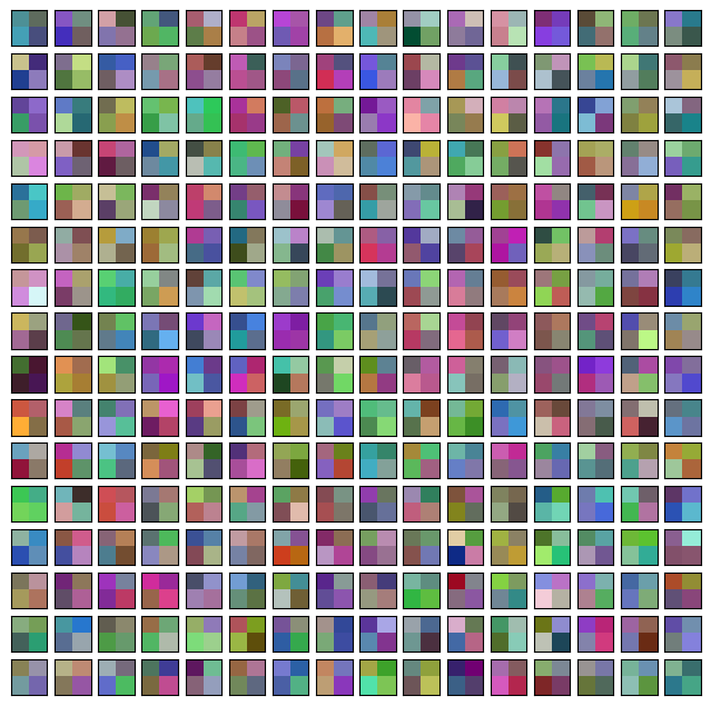
即使我們沒有將網路訓練到收斂,我們也可以注意到不同的圖塊顯示不同的模式。有些圖塊與其他圖塊有相似之處,而有些則非常不同。這些視覺化在較大的影像尺寸下更為顯著。
同樣地,我們可以視覺化原始卷積核心。這可以幫助我們了解給定核心接收的模式。
# First, print the indices of the convolution layers that are not
# pointwise convolutions.
for i, layer in enumerate(conv_mixer_model.layers):
    if isinstance(layer, layers.DepthwiseConv2D):
        if layer.get_config()["kernel_size"] == (5, 5):
            print(i, layer)

idx = 26  # Taking a kernel from the middle of the network.

kernel = conv_mixer_model.layers[idx].get_weights()[0]
kernel = np.expand_dims(kernel.squeeze(), axis=2)
visualization_plot(kernel)
5 <DepthwiseConv2D name=depthwise_conv2d, built=True>
12 <DepthwiseConv2D name=depthwise_conv2d_1, built=True>
19 <DepthwiseConv2D name=depthwise_conv2d_2, built=True>
26 <DepthwiseConv2D name=depthwise_conv2d_3, built=True>
33 <DepthwiseConv2D name=depthwise_conv2d_4, built=True>
40 <DepthwiseConv2D name=depthwise_conv2d_5, built=True>
47 <DepthwiseConv2D name=depthwise_conv2d_6, built=True>
54 <DepthwiseConv2D name=depthwise_conv2d_7, built=True>
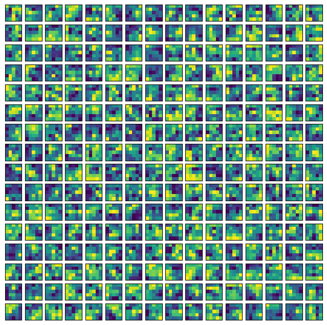
我們看到核心中的不同濾波器具有不同的局部跨度,並且這種模式可能會隨著更多的訓練而演變。
最後說明
最近出現了一種趨勢,將卷積與其他與資料無關的操作(如自我注意)融合在一起。以下工作沿著這個研究方向進行
- ConViT (d'Ascoli 等人)
- CCT (Hassani 等人)
- CoAtNet (Dai 等人)