用於單張影像超解析度的增強型深度殘差網路
作者: Gitesh Chawda
建立日期 2022/04/07
上次修改日期 2024/08/27
說明: 在 DIV2K 資料集上訓練 EDSR 模型。

簡介
在此範例中,我們實作了 Bee Lim、Sanghyun Son、Heewon Kim、Seungjun Nah 和 Kyoung Mu Lee 的用於單張影像超解析度的增強型深度殘差網路 (EDSR)。
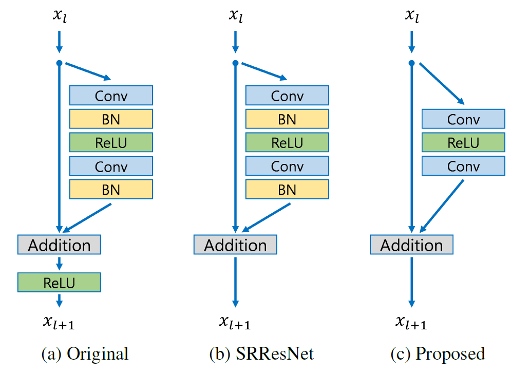
EDSR 架構基於 SRResNet 架構,並由多個殘差區塊組成。它使用恆定縮放層而不是批次標準化層來產生一致的結果(輸入和輸出具有相似的分佈,因此正規化中間特徵可能不是理想的)。作者沒有使用 L2 損失(均方誤差),而是採用了 L1 損失(平均絕對誤差),這在經驗上表現更好。
我們的實作僅包含 16 個具有 64 個通道的殘差區塊。
或者,如 Keras 範例使用高效子像素 CNN 進行影像超解析度中所示,您可以使用 ESPCN 模型進行超解析度。根據調查論文,EDSR 是基於 PSNR 分數的前五名表現最佳的超解析度方法之一。但是,它比其他方法具有更多的參數,並且需要更多的計算能力。它的 PSNR 值 (≈34db) 略高於 ESPCN (≈32db)。根據調查論文,EDSR 的效能優於 ESPCN。
比較圖: 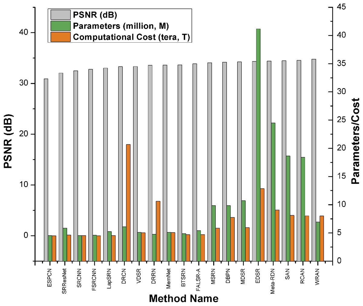
匯入
import os

os.environ["KERAS_BACKEND"] = "tensorflow"

import numpy as np
import tensorflow as tf
import tensorflow_datasets as tfds
import matplotlib.pyplot as plt

import keras
from keras import layers
from keras import ops

AUTOTUNE = tf.data.AUTOTUNE
下載訓練資料集
我們使用 DIV2K 資料集,這是一個著名的單張影像超解析度資料集,其中包含 1,000 張具有各種降級場景的影像,分為 800 張用於訓練、100 張用於驗證和 100 張用於測試。我們使用 4 倍雙立方降採樣影像作為我們的「低品質」參考。
# Download DIV2K from TF Datasets
# Using bicubic 4x degradation type
div2k_data = tfds.image.Div2k(config="bicubic_x4")
div2k_data.download_and_prepare()

# Taking train data from div2k_data object
train = div2k_data.as_dataset(split="train", as_supervised=True)
train_cache = train.cache()
# Validation data
val = div2k_data.as_dataset(split="validation", as_supervised=True)
val_cache = val.cache()
翻轉、裁剪和調整影像大小
def flip_left_right(lowres_img, highres_img):
    """Flips Images to left and right."""

    # Outputs random values from a uniform distribution in between 0 to 1
    rn = keras.random.uniform(shape=(), maxval=1)
    # If rn is less than 0.5 it returns original lowres_img and highres_img
    # If rn is greater than 0.5 it returns flipped image
    return ops.cond(
        rn < 0.5,
        lambda: (lowres_img, highres_img),
        lambda: (
            ops.flip(lowres_img),
            ops.flip(highres_img),
        ),
    )


def random_rotate(lowres_img, highres_img):
    """Rotates Images by 90 degrees."""

    # Outputs random values from uniform distribution in between 0 to 4
    rn = ops.cast(
        keras.random.uniform(shape=(), maxval=4, dtype="float32"), dtype="int32"
    )
    # Here rn signifies number of times the image(s) are rotated by 90 degrees
    return tf.image.rot90(lowres_img, rn), tf.image.rot90(highres_img, rn)


def random_crop(lowres_img, highres_img, hr_crop_size=96, scale=4):
    """Crop images.

    low resolution images: 24x24
    high resolution images: 96x96
    """
    lowres_crop_size = hr_crop_size // scale  # 96//4=24
    lowres_img_shape = ops.shape(lowres_img)[:2]  # (height,width)

    lowres_width = ops.cast(
        keras.random.uniform(
            shape=(), maxval=lowres_img_shape[1] - lowres_crop_size + 1, dtype="float32"
        ),
        dtype="int32",
    )
    lowres_height = ops.cast(
        keras.random.uniform(
            shape=(), maxval=lowres_img_shape[0] - lowres_crop_size + 1, dtype="float32"
        ),
        dtype="int32",
    )

    highres_width = lowres_width * scale
    highres_height = lowres_height * scale

    lowres_img_cropped = lowres_img[
        lowres_height : lowres_height + lowres_crop_size,
        lowres_width : lowres_width + lowres_crop_size,
    ]  # 24x24
    highres_img_cropped = highres_img[
        highres_height : highres_height + hr_crop_size,
        highres_width : highres_width + hr_crop_size,
    ]  # 96x96

    return lowres_img_cropped, highres_img_cropped
準備一個 tf.data.Dataset 物件
我們使用隨機水平翻轉和 90 度旋轉來增強訓練資料。
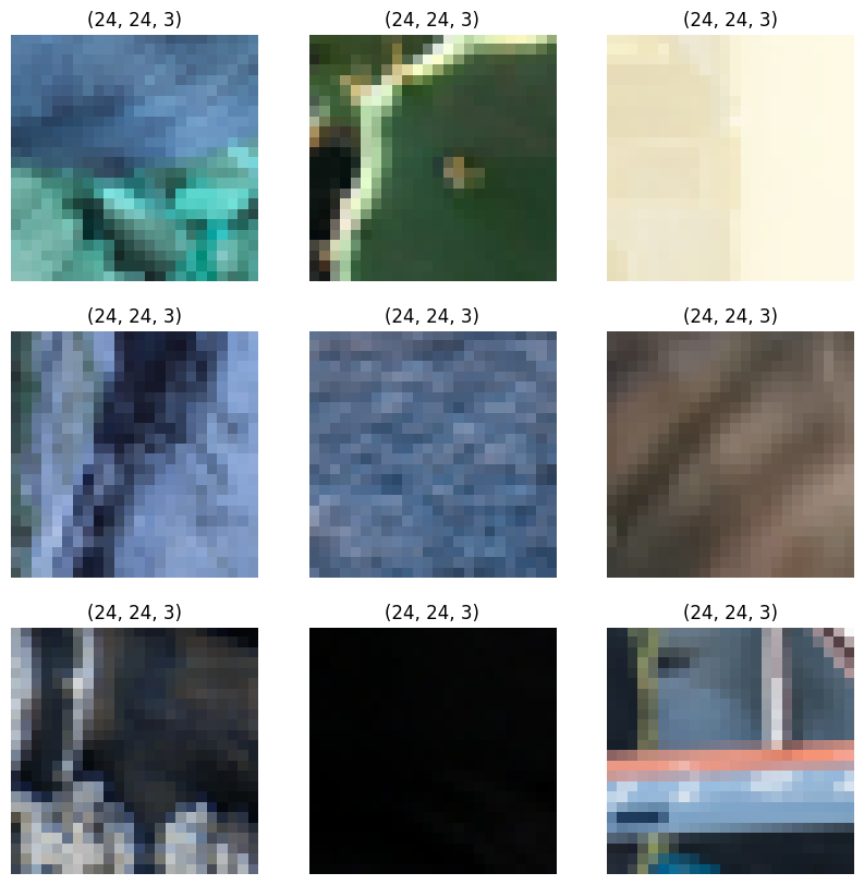
作為低解析度影像,我們使用 24x24 RGB 輸入區塊。
def dataset_object(dataset_cache, training=True):
    ds = dataset_cache
    ds = ds.map(
        lambda lowres, highres: random_crop(lowres, highres, scale=4),
        num_parallel_calls=AUTOTUNE,
    )

    if training:
        ds = ds.map(random_rotate, num_parallel_calls=AUTOTUNE)
        ds = ds.map(flip_left_right, num_parallel_calls=AUTOTUNE)
    # Batching Data
    ds = ds.batch(16)

    if training:
        # Repeating Data, so that cardinality if dataset becomes infinte
        ds = ds.repeat()
    # prefetching allows later images to be prepared while the current image is being processed
    ds = ds.prefetch(buffer_size=AUTOTUNE)
    return ds


train_ds = dataset_object(train_cache, training=True)
val_ds = dataset_object(val_cache, training=False)
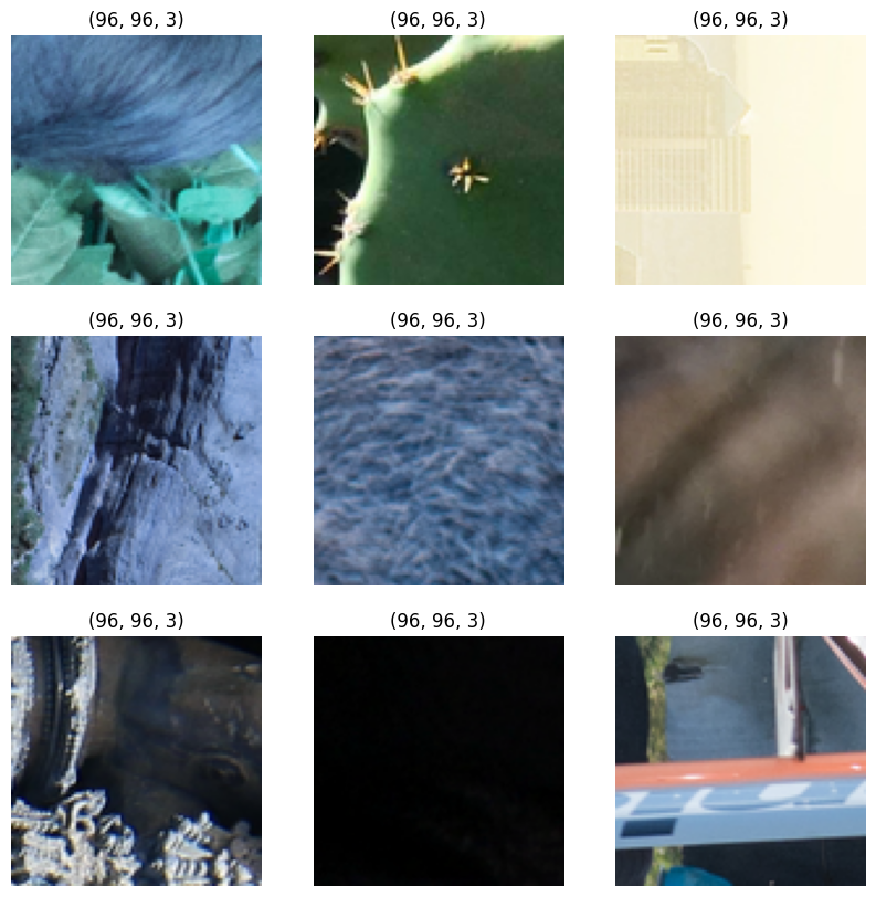
視覺化資料
讓我們視覺化一些範例影像
lowres, highres = next(iter(train_ds))

# High Resolution Images
plt.figure(figsize=(10, 10))
for i in range(9):
    ax = plt.subplot(3, 3, i + 1)
    plt.imshow(highres[i].numpy().astype("uint8"))
    plt.title(highres[i].shape)
    plt.axis("off")

# Low Resolution Images
plt.figure(figsize=(10, 10))
for i in range(9):
    ax = plt.subplot(3, 3, i + 1)
    plt.imshow(lowres[i].numpy().astype("uint8"))
    plt.title(lowres[i].shape)
    plt.axis("off")


def PSNR(super_resolution, high_resolution):
    """Compute the peak signal-to-noise ratio, measures quality of image."""
    # Max value of pixel is 255
    psnr_value = tf.image.psnr(high_resolution, super_resolution, max_val=255)[0]
    return psnr_value
建構模型
在論文中,作者訓練了三個模型:EDSR、MDSR 和基準模型。在此程式碼範例中,我們僅訓練基準模型。
與具有三個殘差區塊的模型的比較
EDSR 的殘差區塊設計與 ResNet 不同。批次正規化層已被移除(連同最後的 ReLU 激活):由於批次正規化層會正規化特徵,它們會損害輸出值範圍的彈性。因此,移除它們會更好。此外,由於批次正規化層會消耗與前一層卷積層相同的記憶體量,這也有助於減少模型所需的 GPU RAM 量。
class EDSRModel(keras.Model):
    def train_step(self, data):
        # Unpack the data. Its structure depends on your model and
        # on what you pass to `fit()`.
        x, y = data

        with tf.GradientTape() as tape:
            y_pred = self(x, training=True)  # Forward pass
            # Compute the loss value
            # (the loss function is configured in `compile()`)
            loss = self.compiled_loss(y, y_pred, regularization_losses=self.losses)

        # Compute gradients
        trainable_vars = self.trainable_variables
        gradients = tape.gradient(loss, trainable_vars)
        # Update weights
        self.optimizer.apply_gradients(zip(gradients, trainable_vars))
        # Update metrics (includes the metric that tracks the loss)
        self.compiled_metrics.update_state(y, y_pred)
        # Return a dict mapping metric names to current value
        return {m.name: m.result() for m in self.metrics}

    def predict_step(self, x):
        # Adding dummy dimension using tf.expand_dims and converting to float32 using tf.cast
        x = ops.cast(tf.expand_dims(x, axis=0), dtype="float32")
        # Passing low resolution image to model
        super_resolution_img = self(x, training=False)
        # Clips the tensor from min(0) to max(255)
        super_resolution_img = ops.clip(super_resolution_img, 0, 255)
        # Rounds the values of a tensor to the nearest integer
        super_resolution_img = ops.round(super_resolution_img)
        # Removes dimensions of size 1 from the shape of a tensor and converting to uint8
        super_resolution_img = ops.squeeze(
            ops.cast(super_resolution_img, dtype="uint8"), axis=0
        )
        return super_resolution_img


# Residual Block
def ResBlock(inputs):
    x = layers.Conv2D(64, 3, padding="same", activation="relu")(inputs)
    x = layers.Conv2D(64, 3, padding="same")(x)
    x = layers.Add()([inputs, x])
    return x


# Upsampling Block
def Upsampling(inputs, factor=2, **kwargs):
    x = layers.Conv2D(64 * (factor**2), 3, padding="same", **kwargs)(inputs)
    x = layers.Lambda(lambda x: tf.nn.depth_to_space(x, block_size=factor))(x)
    x = layers.Conv2D(64 * (factor**2), 3, padding="same", **kwargs)(x)
    x = layers.Lambda(lambda x: tf.nn.depth_to_space(x, block_size=factor))(x)
    return x


def make_model(num_filters, num_of_residual_blocks):
    # Flexible Inputs to input_layer
    input_layer = layers.Input(shape=(None, None, 3))
    # Scaling Pixel Values
    x = layers.Rescaling(scale=1.0 / 255)(input_layer)
    x = x_new = layers.Conv2D(num_filters, 3, padding="same")(x)

    # 16 residual blocks
    for _ in range(num_of_residual_blocks):
        x_new = ResBlock(x_new)

    x_new = layers.Conv2D(num_filters, 3, padding="same")(x_new)
    x = layers.Add()([x, x_new])

    x = Upsampling(x)
    x = layers.Conv2D(3, 3, padding="same")(x)

    output_layer = layers.Rescaling(scale=255)(x)
    return EDSRModel(input_layer, output_layer)


model = make_model(num_filters=64, num_of_residual_blocks=16)
訓練模型
# Using adam optimizer with initial learning rate as 1e-4, changing learning rate after 5000 steps to 5e-5
optim_edsr = keras.optimizers.Adam(
    learning_rate=keras.optimizers.schedules.PiecewiseConstantDecay(
        boundaries=[5000], values=[1e-4, 5e-5]
    )
)
# Compiling model with loss as mean absolute error(L1 Loss) and metric as psnr
model.compile(optimizer=optim_edsr, loss="mae", metrics=[PSNR])
# Training for more epochs will improve results
model.fit(train_ds, epochs=100, steps_per_epoch=200, validation_data=val_ds)
Epoch 1/100
 200/200 ━━━━━━━━━━━━━━━━━━━━ 117s 472ms/step - psnr: 8.7874 - loss: 85.1546 - val_loss: 17.4624 - val_psnr: 8.7008
Epoch 10/100
200/200 ━━━━━━━━━━━━━━━━━━━━ 58s 288ms/step - psnr: 8.9519 - loss: 94.4611 - val_loss: 8.6002 - val_psnr: 6.4303
Epoch 20/100
200/200 ━━━━━━━━━━━━━━━━━━━━ 52s 261ms/step - psnr: 8.5120 - loss: 95.5767 - val_loss: 8.7330 - val_psnr: 6.3106
Epoch 30/100
 200/200 ━━━━━━━━━━━━━━━━━━━━ 53s 262ms/step - psnr: 8.6051 - loss: 96.1541 - val_loss: 7.5442 - val_psnr: 7.9715
Epoch 40/100
200/200 ━━━━━━━━━━━━━━━━━━━━ 53s 263ms/step - psnr: 8.7405 - loss: 96.8159 - val_loss: 7.2734 - val_psnr: 7.6312
Epoch 50/100
 200/200 ━━━━━━━━━━━━━━━━━━━━ 52s 259ms/step - psnr: 8.7648 - loss: 95.7817 - val_loss: 8.1772 - val_psnr: 7.1330
Epoch 60/100
200/200 ━━━━━━━━━━━━━━━━━━━━ 53s 264ms/step - psnr: 8.8651 - loss: 95.4793 - val_loss: 7.6550 - val_psnr: 7.2298
Epoch 70/100
200/200 ━━━━━━━━━━━━━━━━━━━━ 53s 263ms/step - psnr: 8.8489 - loss: 94.5993 - val_loss: 7.4607 - val_psnr: 6.6841
Epoch 80/100
200/200 ━━━━━━━━━━━━━━━━━━━━ 53s 263ms/step - psnr: 8.3046 - loss: 97.3796 - val_loss: 8.1050 - val_psnr: 8.0714
Epoch 90/100
200/200 ━━━━━━━━━━━━━━━━━━━━ 53s 264ms/step - psnr: 7.9295 - loss: 96.0314 - val_loss: 7.1515 - val_psnr: 6.8712
Epoch 100/100
 200/200 ━━━━━━━━━━━━━━━━━━━━ 53s 263ms/step - psnr: 8.1666 - loss: 94.9792 - val_loss: 6.6524 - val_psnr: 6.5423


<keras.src.callbacks.history.History at 0x7fc1e8dd6890>
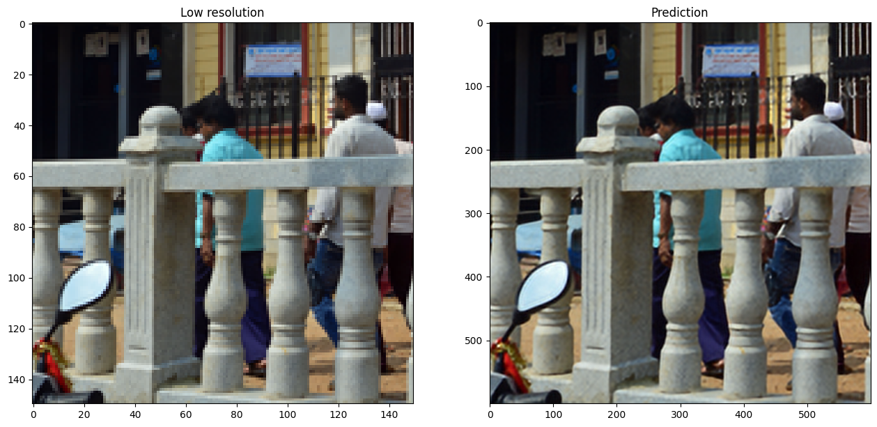
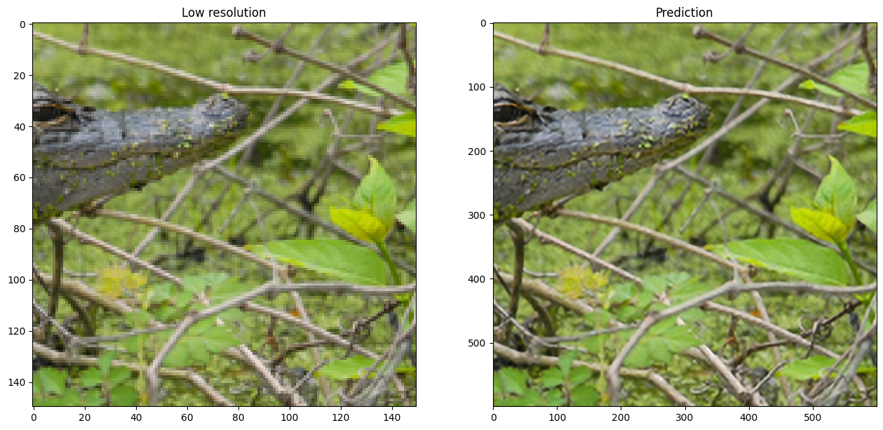
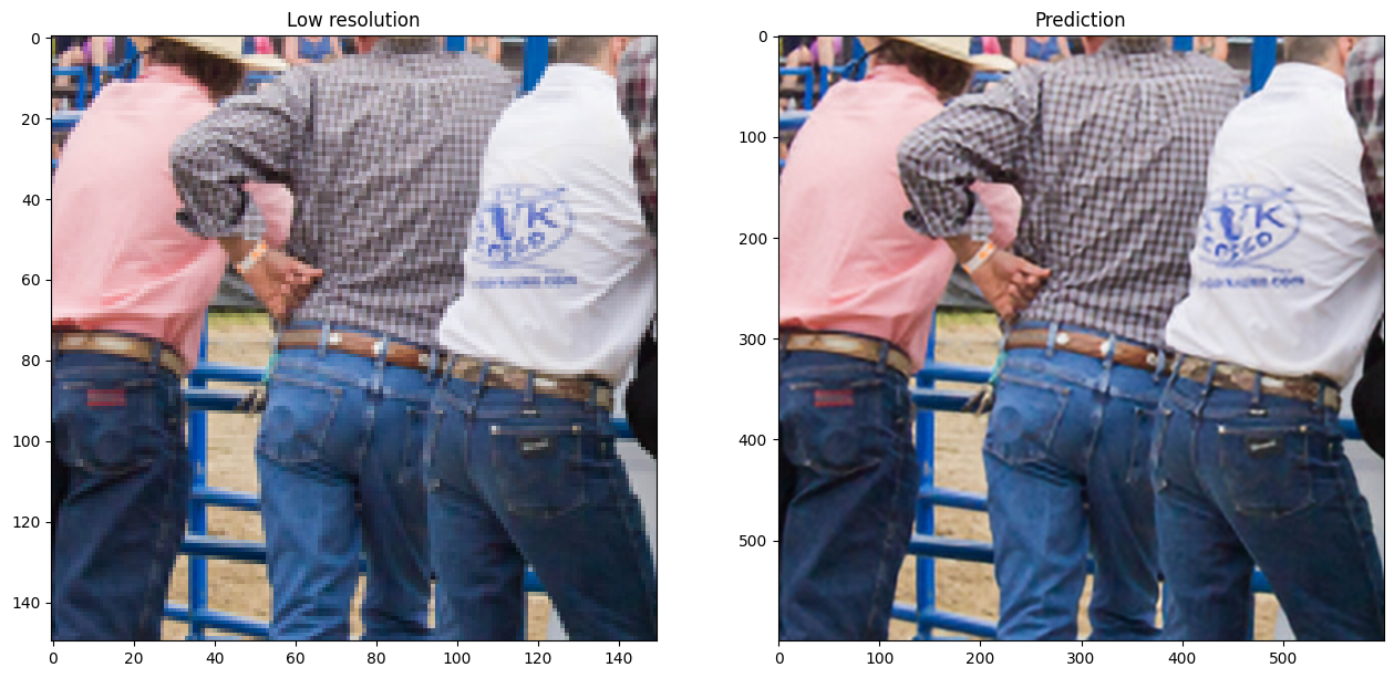
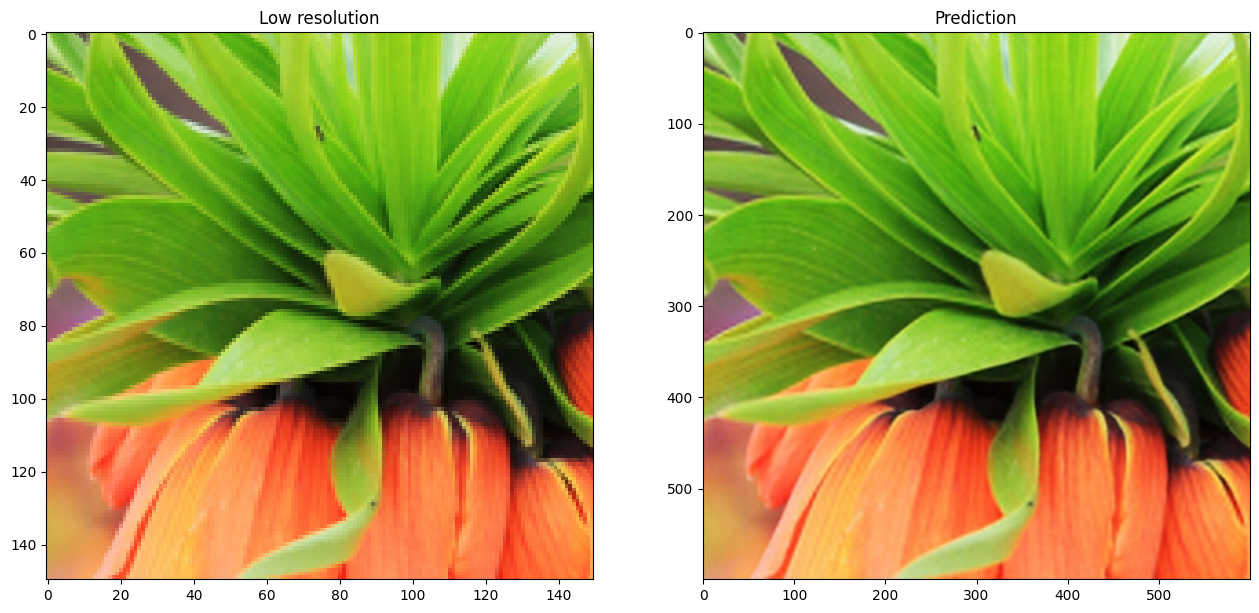
在新圖像上運行推論並繪製結果
def plot_results(lowres, preds):
    """
    Displays low resolution image and super resolution image
    """
    plt.figure(figsize=(24, 14))
    plt.subplot(132), plt.imshow(lowres), plt.title("Low resolution")
    plt.subplot(133), plt.imshow(preds), plt.title("Prediction")
    plt.show()


for lowres, highres in val.take(10):
    lowres = tf.image.random_crop(lowres, (150, 150, 3))
    preds = model.predict_step(lowres)
    plot_results(lowres, preds)
最終評論
在這個範例中,我們實作了 EDSR 模型(用於單張影像超解析度的增強型深度殘差網路)。您可以透過訓練模型更多個 epoch 來提高模型準確性,以及使用具有混合降級因子的更多樣化輸入來訓練模型,以便能夠處理更廣泛的真實世界圖像。
您還可以透過實作 EDSR+ 或 MDSR(多尺度超解析度)和 MDSR+ 來改進給定的基準 EDSR 模型,這些模型在同一篇論文中提出。