手寫辨識
作者: A_K_Nain, Sayak Paul
建立日期 2021/08/16
最後修改日期 2024/09/01
描述: 訓練具有可變長度序列的手寫辨識模型。

簡介
此範例展示如何將 驗證碼 OCR 範例擴展到 IAM 資料集,該資料集具有可變長度的真實目標。資料集中的每個樣本都是一些手寫文字的圖片,其對應的目標是圖片中存在的字串。IAM 資料集廣泛用於許多 OCR 基準測試,因此我們希望此範例可以作為建構 OCR 系統的良好起點。
資料收集
!wget -q https://github.com/sayakpaul/Handwriting-Recognizer-in-Keras/releases/download/v1.0.0/IAM_Words.zip
!unzip -qq IAM_Words.zip
!
!mkdir data
!mkdir data/words
!tar -xf IAM_Words/words.tgz -C data/words
!mv IAM_Words/words.txt data
預覽資料集的組織方式。以「#」開頭的行僅為中繼資料資訊。
!head -20 data/words.txt
#--- words.txt ---------------------------------------------------------------#
#
# iam database word information
#
# format: a01-000u-00-00 ok 154 1 408 768 27 51 AT A
#
#     a01-000u-00-00  -> word id for line 00 in form a01-000u
#     ok              -> result of word segmentation
#                            ok: word was correctly
#                            er: segmentation of word can be bad
#
#     154             -> graylevel to binarize the line containing this word
#     1               -> number of components for this word
#     408 768 27 51   -> bounding box around this word in x,y,w,h format
#     AT              -> the grammatical tag for this word, see the
#                        file tagset.txt for an explanation
#     A               -> the transcription for this word
#
a01-000u-00-00 ok 154 408 768 27 51 AT A
a01-000u-00-01 ok 154 507 766 213 48 NN MOVE
匯入
import keras
from keras.layers import StringLookup
from keras import ops
import matplotlib.pyplot as plt
import tensorflow as tf
import numpy as np
import os

np.random.seed(42)
keras.utils.set_random_seed(42)
資料集分割
base_path = "data"
words_list = []

words = open(f"{base_path}/words.txt", "r").readlines()
for line in words:
    if line[0] == "#":
        continue
    if line.split(" ")[1] != "err":  # We don't need to deal with errored entries.
        words_list.append(line)

len(words_list)

np.random.shuffle(words_list)
我們將資料集分割為三個子集,比例為 90:5:5(訓練:驗證:測試)。
split_idx = int(0.9 * len(words_list))
train_samples = words_list[:split_idx]
test_samples = words_list[split_idx:]

val_split_idx = int(0.5 * len(test_samples))
validation_samples = test_samples[:val_split_idx]
test_samples = test_samples[val_split_idx:]

assert len(words_list) == len(train_samples) + len(validation_samples) + len(
    test_samples
)

print(f"Total training samples: {len(train_samples)}")
print(f"Total validation samples: {len(validation_samples)}")
print(f"Total test samples: {len(test_samples)}")
Total training samples: 86810
Total validation samples: 4823
Total test samples: 4823
資料輸入管道
我們首先準備圖片路徑來開始建構資料輸入管道。
base_image_path = os.path.join(base_path, "words")


def get_image_paths_and_labels(samples):
    paths = []
    corrected_samples = []
    for i, file_line in enumerate(samples):
        line_split = file_line.strip()
        line_split = line_split.split(" ")

        # Each line split will have this format for the corresponding image:
        # part1/part1-part2/part1-part2-part3.png
        image_name = line_split[0]
        partI = image_name.split("-")[0]
        partII = image_name.split("-")[1]
        img_path = os.path.join(
            base_image_path, partI, partI + "-" + partII, image_name + ".png"
        )
        if os.path.getsize(img_path):
            paths.append(img_path)
            corrected_samples.append(file_line.split("\n")[0])

    return paths, corrected_samples


train_img_paths, train_labels = get_image_paths_and_labels(train_samples)
validation_img_paths, validation_labels = get_image_paths_and_labels(validation_samples)
test_img_paths, test_labels = get_image_paths_and_labels(test_samples)
然後我們準備真實標籤。
# Find maximum length and the size of the vocabulary in the training data.
train_labels_cleaned = []
characters = set()
max_len = 0

for label in train_labels:
    label = label.split(" ")[-1].strip()
    for char in label:
        characters.add(char)

    max_len = max(max_len, len(label))
    train_labels_cleaned.append(label)

characters = sorted(list(characters))

print("Maximum length: ", max_len)
print("Vocab size: ", len(characters))

# Check some label samples.
train_labels_cleaned[:10]
Maximum length:  21
Vocab size:  78

['sure',
 'he',
 'during',
 'of',
 'booty',
 'gastronomy',
 'boy',
 'The',
 'and',
 'in']
現在我們也清除驗證和測試標籤。
def clean_labels(labels):
    cleaned_labels = []
    for label in labels:
        label = label.split(" ")[-1].strip()
        cleaned_labels.append(label)
    return cleaned_labels


validation_labels_cleaned = clean_labels(validation_labels)
test_labels_cleaned = clean_labels(test_labels)
建構字元詞彙表
Keras 提供了不同的預處理層來處理不同的資料型態。 本指南 提供全面的介紹。我們的範例涉及在字元層級預處理標籤。這表示如果有兩個標籤,例如「cat」和「dog」,則我們的字元詞彙表應為 {a, c, d, g, o, t}(不含任何特殊符號)。我們使用 StringLookup 層來達到此目的。
AUTOTUNE = tf.data.AUTOTUNE

# Mapping characters to integers.
char_to_num = StringLookup(vocabulary=list(characters), mask_token=None)

# Mapping integers back to original characters.
num_to_char = StringLookup(
    vocabulary=char_to_num.get_vocabulary(), mask_token=None, invert=True
)
調整圖片大小而不失真
許多 OCR 模型使用矩形圖片,而不是正方形圖片。當我們可視化資料集中的幾個樣本時,這一點會更加清楚。雖然不考慮長寬比調整正方形圖片大小不會引入大量的失真,但矩形圖片並非如此。但是,將圖片調整為統一大小是進行小批量處理的要求。因此,我們需要執行調整大小的操作,以滿足以下條件
- 長寬比保持不變。
- 圖片的內容不受影響。
def distortion_free_resize(image, img_size):
    w, h = img_size
    image = tf.image.resize(image, size=(h, w), preserve_aspect_ratio=True)

    # Check tha amount of padding needed to be done.
    pad_height = h - ops.shape(image)[0]
    pad_width = w - ops.shape(image)[1]

    # Only necessary if you want to do same amount of padding on both sides.
    if pad_height % 2 != 0:
        height = pad_height // 2
        pad_height_top = height + 1
        pad_height_bottom = height
    else:
        pad_height_top = pad_height_bottom = pad_height // 2

    if pad_width % 2 != 0:
        width = pad_width // 2
        pad_width_left = width + 1
        pad_width_right = width
    else:
        pad_width_left = pad_width_right = pad_width // 2

    image = tf.pad(
        image,
        paddings=[
            [pad_height_top, pad_height_bottom],
            [pad_width_left, pad_width_right],
            [0, 0],
        ],
    )

    image = ops.transpose(image, (1, 0, 2))
    image = tf.image.flip_left_right(image)
    return image
如果我們只是簡單地進行調整大小,那麼圖片看起來會像這樣

請注意,這種調整大小會如何引入不必要的拉伸。
將實用程式組合在一起
batch_size = 64
padding_token = 99
image_width = 128
image_height = 32


def preprocess_image(image_path, img_size=(image_width, image_height)):
    image = tf.io.read_file(image_path)
    image = tf.image.decode_png(image, 1)
    image = distortion_free_resize(image, img_size)
    image = ops.cast(image, tf.float32) / 255.0
    return image


def vectorize_label(label):
    label = char_to_num(tf.strings.unicode_split(label, input_encoding="UTF-8"))
    length = ops.shape(label)[0]
    pad_amount = max_len - length
    label = tf.pad(label, paddings=[[0, pad_amount]], constant_values=padding_token)
    return label


def process_images_labels(image_path, label):
    image = preprocess_image(image_path)
    label = vectorize_label(label)
    return {"image": image, "label": label}


def prepare_dataset(image_paths, labels):
    dataset = tf.data.Dataset.from_tensor_slices((image_paths, labels)).map(
        process_images_labels, num_parallel_calls=AUTOTUNE
    )
    return dataset.batch(batch_size).cache().prefetch(AUTOTUNE)
準備 tf.data.Dataset 物件
train_ds = prepare_dataset(train_img_paths, train_labels_cleaned)
validation_ds = prepare_dataset(validation_img_paths, validation_labels_cleaned)
test_ds = prepare_dataset(test_img_paths, test_labels_cleaned)
視覺化一些樣本
for data in train_ds.take(1):
    images, labels = data["image"], data["label"]

    _, ax = plt.subplots(4, 4, figsize=(15, 8))

    for i in range(16):
        img = images[i]
        img = tf.image.flip_left_right(img)
        img = ops.transpose(img, (1, 0, 2))
        img = (img * 255.0).numpy().clip(0, 255).astype(np.uint8)
        img = img[:, :, 0]

        # Gather indices where label!= padding_token.
        label = labels[i]
        indices = tf.gather(label, tf.where(tf.math.not_equal(label, padding_token)))
        # Convert to string.
        label = tf.strings.reduce_join(num_to_char(indices))
        label = label.numpy().decode("utf-8")

        ax[i // 4, i % 4].imshow(img, cmap="gray")
        ax[i // 4, i % 4].set_title(label)
        ax[i // 4, i % 4].axis("off")


plt.show()
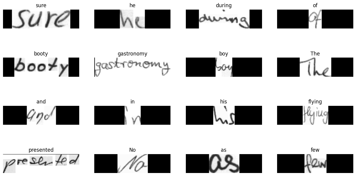
您會注意到原始影像的內容盡可能地保持真實,並已相應地進行填充。
模型
我們的模型將使用 CTC 損失作為端點層。如需詳細了解 CTC 損失,請參考這篇文章。
class CTCLayer(keras.layers.Layer):
    def __init__(self, name=None):
        super().__init__(name=name)
        self.loss_fn = tf.keras.backend.ctc_batch_cost

    def call(self, y_true, y_pred):
        batch_len = ops.cast(ops.shape(y_true)[0], dtype="int64")
        input_length = ops.cast(ops.shape(y_pred)[1], dtype="int64")
        label_length = ops.cast(ops.shape(y_true)[1], dtype="int64")

        input_length = input_length * ops.ones(shape=(batch_len, 1), dtype="int64")
        label_length = label_length * ops.ones(shape=(batch_len, 1), dtype="int64")
        loss = self.loss_fn(y_true, y_pred, input_length, label_length)
        self.add_loss(loss)

        # At test time, just return the computed predictions.
        return y_pred


def build_model():
    # Inputs to the model
    input_img = keras.Input(shape=(image_width, image_height, 1), name="image")
    labels = keras.layers.Input(name="label", shape=(None,))

    # First conv block.
    x = keras.layers.Conv2D(
        32,
        (3, 3),
        activation="relu",
        kernel_initializer="he_normal",
        padding="same",
        name="Conv1",
    )(input_img)
    x = keras.layers.MaxPooling2D((2, 2), name="pool1")(x)

    # Second conv block.
    x = keras.layers.Conv2D(
        64,
        (3, 3),
        activation="relu",
        kernel_initializer="he_normal",
        padding="same",
        name="Conv2",
    )(x)
    x = keras.layers.MaxPooling2D((2, 2), name="pool2")(x)

    # We have used two max pool with pool size and strides 2.
    # Hence, downsampled feature maps are 4x smaller. The number of
    # filters in the last layer is 64. Reshape accordingly before
    # passing the output to the RNN part of the model.
    new_shape = ((image_width // 4), (image_height // 4) * 64)
    x = keras.layers.Reshape(target_shape=new_shape, name="reshape")(x)
    x = keras.layers.Dense(64, activation="relu", name="dense1")(x)
    x = keras.layers.Dropout(0.2)(x)

    # RNNs.
    x = keras.layers.Bidirectional(
        keras.layers.LSTM(128, return_sequences=True, dropout=0.25)
    )(x)
    x = keras.layers.Bidirectional(
        keras.layers.LSTM(64, return_sequences=True, dropout=0.25)
    )(x)

    # +2 is to account for the two special tokens introduced by the CTC loss.
    # The recommendation comes here: https://git.io/J0eXP.
    x = keras.layers.Dense(
        len(char_to_num.get_vocabulary()) + 2, activation="softmax", name="dense2"
    )(x)

    # Add CTC layer for calculating CTC loss at each step.
    output = CTCLayer(name="ctc_loss")(labels, x)

    # Define the model.
    model = keras.models.Model(
        inputs=[input_img, labels], outputs=output, name="handwriting_recognizer"
    )
    # Optimizer.
    opt = keras.optimizers.Adam()
    # Compile the model and return.
    model.compile(optimizer=opt)
    return model


# Get the model.
model = build_model()
model.summary()
Model: "handwriting_recognizer"
┏━━━━━━━━━━━━━━━━━━━━━┳━━━━━━━━━━━━━━━━━━━┳━━━━━━━━━━━━┳━━━━━━━━━━━━━━━━━━━┓
┃ Layer (type)        ┃ Output Shape      ┃    Param # ┃ Connected to      ┃
┡━━━━━━━━━━━━━━━━━━━━━╇━━━━━━━━━━━━━━━━━━━╇━━━━━━━━━━━━╇━━━━━━━━━━━━━━━━━━━┩
│ image (InputLayer)  │ (None, 128, 32,   │          0 │ -                 │
│                     │ 1)                │            │                   │
├─────────────────────┼───────────────────┼────────────┼───────────────────┤
│ Conv1 (Conv2D)      │ (None, 128, 32,   │        320 │ image[0][0]       │
│                     │ 32)               │            │                   │
├─────────────────────┼───────────────────┼────────────┼───────────────────┤
│ pool1               │ (None, 64, 16,    │          0 │ Conv1[0][0]       │
│ (MaxPooling2D)      │ 32)               │            │                   │
├─────────────────────┼───────────────────┼────────────┼───────────────────┤
│ Conv2 (Conv2D)      │ (None, 64, 16,    │     18,496 │ pool1[0][0]       │
│                     │ 64)               │            │                   │
├─────────────────────┼───────────────────┼────────────┼───────────────────┤
│ pool2               │ (None, 32, 8, 64) │          0 │ Conv2[0][0]       │
│ (MaxPooling2D)      │                   │            │                   │
├─────────────────────┼───────────────────┼────────────┼───────────────────┤
│ reshape (Reshape)   │ (None, 32, 512)   │          0 │ pool2[0][0]       │
├─────────────────────┼───────────────────┼────────────┼───────────────────┤
│ dense1 (Dense)      │ (None, 32, 64)    │     32,832 │ reshape[0][0]     │
├─────────────────────┼───────────────────┼────────────┼───────────────────┤
│ dropout (Dropout)   │ (None, 32, 64)    │          0 │ dense1[0][0]      │
├─────────────────────┼───────────────────┼────────────┼───────────────────┤
│ bidirectional       │ (None, 32, 256)   │    197,632 │ dropout[0][0]     │
│ (Bidirectional)     │                   │            │                   │
├─────────────────────┼───────────────────┼────────────┼───────────────────┤
│ bidirectional_1     │ (None, 32, 128)   │    164,352 │ bidirectional[0]… │
│ (Bidirectional)     │                   │            │                   │
├─────────────────────┼───────────────────┼────────────┼───────────────────┤
│ label (InputLayer)  │ (None, None)      │          0 │ -                 │
├─────────────────────┼───────────────────┼────────────┼───────────────────┤
│ dense2 (Dense)      │ (None, 32, 81)    │     10,449 │ bidirectional_1[… │
├─────────────────────┼───────────────────┼────────────┼───────────────────┤
│ ctc_loss (CTCLayer) │ (None, 32, 81)    │          0 │ label[0][0],      │
│                     │                   │            │ dense2[0][0]      │
└─────────────────────┴───────────────────┴────────────┴───────────────────┘
Total params: 424,081 (1.62 MB)
Trainable params: 424,081 (1.62 MB)
Non-trainable params: 0 (0.00 B)
評估指標
編輯距離是評估 OCR 模型最廣泛使用的指標。在本節中,我們將實作它並將其用作回調,以監控我們的模型。
為了方便起見,我們先將驗證影像及其標籤分開。
validation_images = []
validation_labels = []

for batch in validation_ds:
    validation_images.append(batch["image"])
    validation_labels.append(batch["label"])
現在,我們建立一個回調來監控編輯距離。
def calculate_edit_distance(labels, predictions):
    # Get a single batch and convert its labels to sparse tensors.
    saprse_labels = ops.cast(tf.sparse.from_dense(labels), dtype=tf.int64)

    # Make predictions and convert them to sparse tensors.
    input_len = np.ones(predictions.shape[0]) * predictions.shape[1]
    predictions_decoded = keras.ops.nn.ctc_decode(
        predictions, sequence_lengths=input_len
    )[0][0][:, :max_len]
    sparse_predictions = ops.cast(
        tf.sparse.from_dense(predictions_decoded), dtype=tf.int64
    )

    # Compute individual edit distances and average them out.
    edit_distances = tf.edit_distance(
        sparse_predictions, saprse_labels, normalize=False
    )
    return tf.reduce_mean(edit_distances)


class EditDistanceCallback(keras.callbacks.Callback):
    def __init__(self, pred_model):
        super().__init__()
        self.prediction_model = pred_model

    def on_epoch_end(self, epoch, logs=None):
        edit_distances = []

        for i in range(len(validation_images)):
            labels = validation_labels[i]
            predictions = self.prediction_model.predict(validation_images[i])
            edit_distances.append(calculate_edit_distance(labels, predictions).numpy())

        print(
            f"Mean edit distance for epoch {epoch + 1}: {np.mean(edit_distances):.4f}"
        )
訓練
現在我們準備開始模型訓練。
epochs = 10  # To get good results this should be at least 50.

model = build_model()
prediction_model = keras.models.Model(
    model.get_layer(name="image").output, model.get_layer(name="dense2").output
)
edit_distance_callback = EditDistanceCallback(prediction_model)

# Train the model.
history = model.fit(
    train_ds,
    validation_data=validation_ds,
    epochs=epochs,
    callbacks=[edit_distance_callback],
)
Epoch 1/10
  1357/1357 ━━━━━━━━━━━━━━━━━━━━ 216s 157ms/step - loss: 1068.7206 - val_loss: 762.4462

Epoch 2/10
  1357/1357 ━━━━━━━━━━━━━━━━━━━━ 215s 158ms/step - loss: 735.8929 - val_loss: 627.9722

Epoch 3/10
  1357/1357 ━━━━━━━━━━━━━━━━━━━━ 211s 155ms/step - loss: 624.9929 - val_loss: 540.8905

Epoch 4/10
  1357/1357 ━━━━━━━━━━━━━━━━━━━━ 208s 153ms/step - loss: 544.2097 - val_loss: 446.0919

Epoch 5/10
  1357/1357 ━━━━━━━━━━━━━━━━━━━━ 213s 157ms/step - loss: 459.0329 - val_loss: 347.1689

Epoch 6/10
  1357/1357 ━━━━━━━━━━━━━━━━━━━━ 210s 155ms/step - loss: 378.6367 - val_loss: 287.1726

Epoch 7/10
  1357/1357 ━━━━━━━━━━━━━━━━━━━━ 211s 155ms/step - loss: 325.4126 - val_loss: 250.3677

Epoch 8/10
  1357/1357 ━━━━━━━━━━━━━━━━━━━━ 209s 154ms/step - loss: 289.2796 - val_loss: 224.4595

Epoch 9/10
  1357/1357 ━━━━━━━━━━━━━━━━━━━━ 209s 154ms/step - loss: 264.0461 - val_loss: 205.5910

Epoch 10/10
  1357/1357 ━━━━━━━━━━━━━━━━━━━━ 208s 153ms/step - loss: 245.5216 - val_loss: 195.7952
</div>

---
## Inference


```python

# A utility function to decode the output of the network.
def decode_batch_predictions(pred):
    input_len = np.ones(pred.shape[0]) * pred.shape[1]
    # Use greedy search. For complex tasks, you can use beam search.
    results = keras.ops.nn.ctc_decode(pred, sequence_lengths=input_len)[0][0][
        :, :max_len
    ]
    # Iterate over the results and get back the text.
    output_text = []
    for res in results:
        res = tf.gather(res, tf.where(tf.math.not_equal(res, -1)))
        res = (
            tf.strings.reduce_join(num_to_char(res))
            .numpy()
            .decode("utf-8")
            .replace("[UNK]", "")
        )
        output_text.append(res)
    return output_text


#  Let's check results on some test samples.
for batch in test_ds.take(1):
    batch_images = batch["image"]
    _, ax = plt.subplots(4, 4, figsize=(15, 8))

    preds = prediction_model.predict(batch_images)
    pred_texts = decode_batch_predictions(preds)

    for i in range(16):
        img = batch_images[i]
        img = tf.image.flip_left_right(img)
        img = ops.transpose(img, (1, 0, 2))
        img = (img * 255.0).numpy().clip(0, 255).astype(np.uint8)
        img = img[:, :, 0]

        title = f"Prediction: {pred_texts[i]}"
        ax[i // 4, i % 4].imshow(img, cmap="gray")
        ax[i // 4, i % 4].set_title(title)
        ax[i // 4, i % 4].axis("off")

plt.show()