使用遷移學習進行關鍵點檢測
作者: Sayak Paul,由 Muhammad Anas Raza 轉換為 Keras 3
建立日期 2021/05/02
上次修改日期 2023/07/19
說明: 使用數據增強和遷移學習訓練關鍵點偵測器。

關鍵點檢測包括定位物件的關鍵部位。例如,我們臉部的關鍵部位包括鼻尖、眉毛、眼角等等。這些部位有助於以豐富的功能方式表示底層物件。關鍵點檢測的應用包括姿態估計、人臉檢測等。
在本範例中,我們將使用 StanfordExtra 數據集,並使用遷移學習來建立關鍵點偵測器。此範例需要 TensorFlow 2.4 或更高版本,以及 imgaug 函式庫,可以使用以下命令安裝
!pip install -q -U imgaug
數據收集
StanfordExtra 數據集包含 12,000 張狗的圖像,以及關鍵點和分割地圖。它是由 Stanford dogs 數據集開發而來。可以使用以下命令下載
!wget -q http://vision.stanford.edu/aditya86/ImageNetDogs/images.tar
註解以單個 JSON 檔案的形式提供在 StanfordExtra 數據集中,需要填寫此表單才能存取。作者明確指示使用者不要分享 JSON 檔案,本範例尊重此意願:您應該自行取得 JSON 檔案。
JSON 檔案預期在本機上以 stanfordextra_v12.zip 的形式提供。
下載檔案後,我們可以解壓縮封存檔。
!tar xf images.tar
!unzip -qq ~/stanfordextra_v12.zip
匯入
from keras import layers
import keras

from imgaug.augmentables.kps import KeypointsOnImage
from imgaug.augmentables.kps import Keypoint
import imgaug.augmenters as iaa

from PIL import Image
from sklearn.model_selection import train_test_split
from matplotlib import pyplot as plt
import pandas as pd
import numpy as np
import json
import os
定義超參數
IMG_SIZE = 224
BATCH_SIZE = 64
EPOCHS = 5
NUM_KEYPOINTS = 24 * 2  # 24 pairs each having x and y coordinates
載入數據
作者還提供了中繼資料檔案,指定有關關鍵點的其他資訊,例如顏色資訊、動物姿態名稱等。我們將在 pandas 資料框架中載入此檔案,以提取資訊以用於視覺化目的。
IMG_DIR = "Images"
JSON = "StanfordExtra_V12/StanfordExtra_v12.json"
KEYPOINT_DEF = (
    "https://github.com/benjiebob/StanfordExtra/raw/master/keypoint_definitions.csv"
)

# Load the ground-truth annotations.
with open(JSON) as infile:
    json_data = json.load(infile)

# Set up a dictionary, mapping all the ground-truth information
# with respect to the path of the image.
json_dict = {i["img_path"]: i for i in json_data}
json_dict 的單個條目如下所示
'n02085782-Japanese_spaniel/n02085782_2886.jpg':
{'img_bbox': [205, 20, 116, 201],
 'img_height': 272,
 'img_path': 'n02085782-Japanese_spaniel/n02085782_2886.jpg',
 'img_width': 350,
 'is_multiple_dogs': False,
 'joints': [[108.66666666666667, 252.0, 1],
            [147.66666666666666, 229.0, 1],
            [163.5, 208.5, 1],
            [0, 0, 0],
            [0, 0, 0],
            [0, 0, 0],
            [54.0, 244.0, 1],
            [77.33333333333333, 225.33333333333334, 1],
            [79.0, 196.5, 1],
            [0, 0, 0],
            [0, 0, 0],
            [0, 0, 0],
            [0, 0, 0],
            [0, 0, 0],
            [150.66666666666666, 86.66666666666667, 1],
            [88.66666666666667, 73.0, 1],
            [116.0, 106.33333333333333, 1],
            [109.0, 123.33333333333333, 1],
            [0, 0, 0],
            [0, 0, 0],
            [0, 0, 0],
            [0, 0, 0],
            [0, 0, 0],
            [0, 0, 0]],
 'seg': ...}
在此範例中,我們感興趣的鍵是
img_pathjoints
joints 內總共有 24 個條目。每個條目有 3 個值
- x 坐標
- y 坐標
- 關鍵點的可見性旗標 (1 表示可見,0 表示不可見)
正如我們所見,joints 包含多個 [0, 0, 0] 條目,表示那些關鍵點未被標記。在此範例中,我們將同時考慮不可見和未標記的關鍵點,以便允許迷你批次學習。
# Load the metdata definition file and preview it.
keypoint_def = pd.read_csv(KEYPOINT_DEF)
keypoint_def.head()

# Extract the colours and labels.
colours = keypoint_def["Hex colour"].values.tolist()
colours = ["#" + colour for colour in colours]
labels = keypoint_def["Name"].values.tolist()


# Utility for reading an image and for getting its annotations.
def get_dog(name):
    data = json_dict[name]
    img_data = plt.imread(os.path.join(IMG_DIR, data["img_path"]))
    # If the image is RGBA convert it to RGB.
    if img_data.shape[-1] == 4:
        img_data = img_data.astype(np.uint8)
        img_data = Image.fromarray(img_data)
        img_data = np.array(img_data.convert("RGB"))
    data["img_data"] = img_data

    return data
視覺化數據
現在,我們編寫一個實用函式來視覺化圖像及其關鍵點。
# Parts of this code come from here:
# https://github.com/benjiebob/StanfordExtra/blob/master/demo.ipynb
def visualize_keypoints(images, keypoints):
    fig, axes = plt.subplots(nrows=len(images), ncols=2, figsize=(16, 12))
    [ax.axis("off") for ax in np.ravel(axes)]

    for (ax_orig, ax_all), image, current_keypoint in zip(axes, images, keypoints):
        ax_orig.imshow(image)
        ax_all.imshow(image)

        # If the keypoints were formed by `imgaug` then the coordinates need
        # to be iterated differently.
        if isinstance(current_keypoint, KeypointsOnImage):
            for idx, kp in enumerate(current_keypoint.keypoints):
                ax_all.scatter(
                    [kp.x],
                    [kp.y],
                    c=colours[idx],
                    marker="x",
                    s=50,
                    linewidths=5,
                )
        else:
            current_keypoint = np.array(current_keypoint)
            # Since the last entry is the visibility flag, we discard it.
            current_keypoint = current_keypoint[:, :2]
            for idx, (x, y) in enumerate(current_keypoint):
                ax_all.scatter([x], [y], c=colours[idx], marker="x", s=50, linewidths=5)

    plt.tight_layout(pad=2.0)
    plt.show()


# Select four samples randomly for visualization.
samples = list(json_dict.keys())
num_samples = 4
selected_samples = np.random.choice(samples, num_samples, replace=False)

images, keypoints = [], []

for sample in selected_samples:
    data = get_dog(sample)
    image = data["img_data"]
    keypoint = data["joints"]

    images.append(image)
    keypoints.append(keypoint)

visualize_keypoints(images, keypoints)
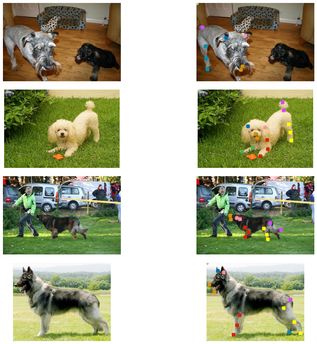
這些圖表顯示我們有大小不一的圖像,這在大多數真實世界情境中是預期的。但是,如果我們調整這些圖像的大小以使其具有統一的形狀 (例如 (224 x 224)),它們的真實註解也會受到影響。如果我們對圖像套用任何幾何變換 (例如水平翻轉),也是如此。幸運的是,imgaug 提供了可以處理此問題的實用程式。在下一節中,我們將編寫一個繼承 keras.utils.Sequence 類別的資料產生器,該產生器使用 imgaug 對批次的數據套用資料增強。
準備數據產生器
class KeyPointsDataset(keras.utils.PyDataset):
    def __init__(self, image_keys, aug, batch_size=BATCH_SIZE, train=True, **kwargs):
        super().__init__(**kwargs)
        self.image_keys = image_keys
        self.aug = aug
        self.batch_size = batch_size
        self.train = train
        self.on_epoch_end()

    def __len__(self):
        return len(self.image_keys) // self.batch_size

    def on_epoch_end(self):
        self.indexes = np.arange(len(self.image_keys))
        if self.train:
            np.random.shuffle(self.indexes)

    def __getitem__(self, index):
        indexes = self.indexes[index * self.batch_size : (index + 1) * self.batch_size]
        image_keys_temp = [self.image_keys[k] for k in indexes]
        (images, keypoints) = self.__data_generation(image_keys_temp)

        return (images, keypoints)

    def __data_generation(self, image_keys_temp):
        batch_images = np.empty((self.batch_size, IMG_SIZE, IMG_SIZE, 3), dtype="int")
        batch_keypoints = np.empty(
            (self.batch_size, 1, 1, NUM_KEYPOINTS), dtype="float32"
        )

        for i, key in enumerate(image_keys_temp):
            data = get_dog(key)
            current_keypoint = np.array(data["joints"])[:, :2]
            kps = []

            # To apply our data augmentation pipeline, we first need to
            # form Keypoint objects with the original coordinates.
            for j in range(0, len(current_keypoint)):
                kps.append(Keypoint(x=current_keypoint[j][0], y=current_keypoint[j][1]))

            # We then project the original image and its keypoint coordinates.
            current_image = data["img_data"]
            kps_obj = KeypointsOnImage(kps, shape=current_image.shape)

            # Apply the augmentation pipeline.
            (new_image, new_kps_obj) = self.aug(image=current_image, keypoints=kps_obj)
            batch_images[i,] = new_image

            # Parse the coordinates from the new keypoint object.
            kp_temp = []
            for keypoint in new_kps_obj:
                kp_temp.append(np.nan_to_num(keypoint.x))
                kp_temp.append(np.nan_to_num(keypoint.y))

            # More on why this reshaping later.
            batch_keypoints[i,] = np.array(kp_temp).reshape(1, 1, 24 * 2)

        # Scale the coordinates to [0, 1] range.
        batch_keypoints = batch_keypoints / IMG_SIZE

        return (batch_images, batch_keypoints)
若要了解如何在 imgaug 中使用關鍵點,請查看 此文件。
定義增強變換
train_aug = iaa.Sequential(
    [
        iaa.Resize(IMG_SIZE, interpolation="linear"),
        iaa.Fliplr(0.3),
        # `Sometimes()` applies a function randomly to the inputs with
        # a given probability (0.3, in this case).
        iaa.Sometimes(0.3, iaa.Affine(rotate=10, scale=(0.5, 0.7))),
    ]
)

test_aug = iaa.Sequential([iaa.Resize(IMG_SIZE, interpolation="linear")])
建立訓練和驗證分割
np.random.shuffle(samples)
train_keys, validation_keys = (
    samples[int(len(samples) * 0.15) :],
    samples[: int(len(samples) * 0.15)],
)
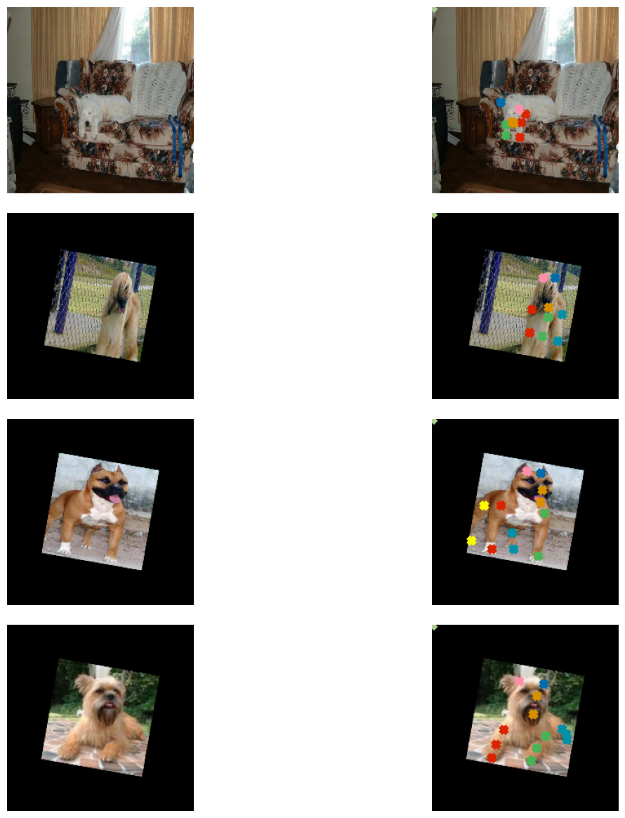
數據產生器調查
train_dataset = KeyPointsDataset(
    train_keys, train_aug, workers=2, use_multiprocessing=True
)
validation_dataset = KeyPointsDataset(
    validation_keys, test_aug, train=False, workers=2, use_multiprocessing=True
)

print(f"Total batches in training set: {len(train_dataset)}")
print(f"Total batches in validation set: {len(validation_dataset)}")

sample_images, sample_keypoints = next(iter(train_dataset))
assert sample_keypoints.max() == 1.0
assert sample_keypoints.min() == 0.0

sample_keypoints = sample_keypoints[:4].reshape(-1, 24, 2) * IMG_SIZE
visualize_keypoints(sample_images[:4], sample_keypoints)
Total batches in training set: 166
Total batches in validation set: 29
模型建構
Stanford dogs 數據集 (StanfordExtra 數據集所依據的) 是使用 ImageNet-1k 數據集建構的。因此,在 ImageNet-1k 數據集上預訓練的模型很可能對此任務有用。我們將使用在此數據集上預訓練的 MobileNetV2 作為骨幹,以從圖像中提取有意義的功能,然後將這些功能傳遞到自訂的迴歸頭以預測坐標。
def get_model():
    # Load the pre-trained weights of MobileNetV2 and freeze the weights
    backbone = keras.applications.MobileNetV2(
        weights="imagenet",
        include_top=False,
        input_shape=(IMG_SIZE, IMG_SIZE, 3),
    )
    backbone.trainable = False

    inputs = layers.Input((IMG_SIZE, IMG_SIZE, 3))
    x = keras.applications.mobilenet_v2.preprocess_input(inputs)
    x = backbone(x)
    x = layers.Dropout(0.3)(x)
    x = layers.SeparableConv2D(
        NUM_KEYPOINTS, kernel_size=5, strides=1, activation="relu"
    )(x)
    outputs = layers.SeparableConv2D(
        NUM_KEYPOINTS, kernel_size=3, strides=1, activation="sigmoid"
    )(x)

    return keras.Model(inputs, outputs, name="keypoint_detector")
我們的自訂網路是全卷積的,這使其比具有全連接密集層的相同版本網路更具參數友善性。
get_model().summary()
Downloading data from https://storage.googleapis.com/tensorflow/keras-applications/mobilenet_v2/mobilenet_v2_weights_tf_dim_ordering_tf_kernels_1.0_224_no_top.h5
 9406464/9406464 ━━━━━━━━━━━━━━━━━━━━ 0s 0us/step
Model: "keypoint_detector"
┏━━━━━━━━━━━━━━━━━━━━━━━━━━━━━━━━━┳━━━━━━━━━━━━━━━━━━━━━━━━━━━┳━━━━━━━━━━━━┓
┃ Layer (type)                    ┃ Output Shape              ┃    Param # ┃
┡━━━━━━━━━━━━━━━━━━━━━━━━━━━━━━━━━╇━━━━━━━━━━━━━━━━━━━━━━━━━━━╇━━━━━━━━━━━━┩
│ input_layer_1 (InputLayer)      │ (None, 224, 224, 3)       │          0 │
├─────────────────────────────────┼───────────────────────────┼────────────┤
│ true_divide (TrueDivide)        │ (None, 224, 224, 3)       │          0 │
├─────────────────────────────────┼───────────────────────────┼────────────┤
│ subtract (Subtract)             │ (None, 224, 224, 3)       │          0 │
├─────────────────────────────────┼───────────────────────────┼────────────┤
│ mobilenetv2_1.00_224            │ (None, 7, 7, 1280)        │  2,257,984 │
│ (Functional)                    │                           │            │
├─────────────────────────────────┼───────────────────────────┼────────────┤
│ dropout (Dropout)               │ (None, 7, 7, 1280)        │          0 │
├─────────────────────────────────┼───────────────────────────┼────────────┤
│ separable_conv2d                │ (None, 3, 3, 48)          │     93,488 │
│ (SeparableConv2D)               │                           │            │
├─────────────────────────────────┼───────────────────────────┼────────────┤
│ separable_conv2d_1              │ (None, 1, 1, 48)          │      2,784 │
│ (SeparableConv2D)               │                           │            │
└─────────────────────────────────┴───────────────────────────┴────────────┘
Total params: 2,354,256 (8.98 MB)
Trainable params: 96,272 (376.06 KB)
Non-trainable params: 2,257,984 (8.61 MB)
請注意網路的輸出形狀:(None, 1, 1, 48)。這就是為什麼我們將座標重新塑形為:batch_keypoints[i, :] = np.array(kp_temp).reshape(1, 1, 24 * 2)。
模型編譯與訓練
在此範例中,我們將只訓練網路五個週期。
model = get_model()
model.compile(loss="mse", optimizer=keras.optimizers.Adam(1e-4))
model.fit(train_dataset, validation_data=validation_dataset, epochs=EPOCHS)
Epoch 1/5
 166/166 ━━━━━━━━━━━━━━━━━━━━ 84s 415ms/step - loss: 0.1110 - val_loss: 0.0959
Epoch 2/5
 166/166 ━━━━━━━━━━━━━━━━━━━━ 79s 472ms/step - loss: 0.0874 - val_loss: 0.0802
Epoch 3/5
 166/166 ━━━━━━━━━━━━━━━━━━━━ 78s 463ms/step - loss: 0.0789 - val_loss: 0.0765
Epoch 4/5
 166/166 ━━━━━━━━━━━━━━━━━━━━ 78s 467ms/step - loss: 0.0769 - val_loss: 0.0731
Epoch 5/5
 166/166 ━━━━━━━━━━━━━━━━━━━━ 77s 464ms/step - loss: 0.0753 - val_loss: 0.0712

<keras.src.callbacks.history.History at 0x7fb5c4299ae0>
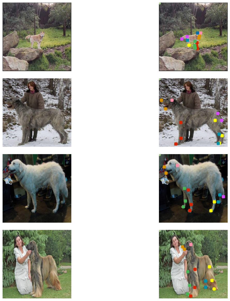
進行預測並視覺化
sample_val_images, sample_val_keypoints = next(iter(validation_dataset))
sample_val_images = sample_val_images[:4]
sample_val_keypoints = sample_val_keypoints[:4].reshape(-1, 24, 2) * IMG_SIZE
predictions = model.predict(sample_val_images).reshape(-1, 24, 2) * IMG_SIZE

# Ground-truth
visualize_keypoints(sample_val_images, sample_val_keypoints)

# Predictions
visualize_keypoints(sample_val_images, predictions)
1/1 ━━━━━━━━━━━━━━━━━━━━ 7s 7s/step
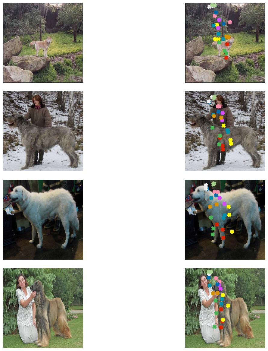
隨著更多訓練,預測可能會有所改善。
更進一步
- 嘗試使用
imgaug中的其他增強轉換,來研究這如何改變結果。 - 在這裡,我們以線性方式從預訓練網路轉移了特徵,也就是我們沒有微調它。我們鼓勵您在這個任務上微調它,並看看是否能提高效能。您也可以嘗試不同的架構,看看它們如何影響最終效能。