在電腦視覺中學習調整大小
作者: Sayak Paul
建立日期 2021/04/30
最後修改日期 2023/12/18
描述: 如何為給定的解析度最佳學習圖像的表示。

普遍認為,如果我們限制視覺模型像人類一樣感知事物,它們的效能可以提高。例如,在這項研究中,Geirhos 等人表明,在 ImageNet-1k 數據集上預訓練的視覺模型偏向於紋理,而人類主要使用形狀描述符來發展共同的感知。但是,這種觀點是否總是適用,尤其是在提高視覺模型的效能方面?
事實證明,情況可能並非總是如此。在訓練視覺模型時,通常會將圖像調整為較低的尺寸((224 x 224)、(299 x 299) 等),以允許小批量學習並保持計算限制。我們通常在此步驟中使用諸如雙線性插值之類的圖像調整大小方法,而調整大小後的圖像對人眼來說不會失去太多感知特性。在學習調整電腦視覺任務的圖像大小中,Talebi 等人表明,如果我們嘗試針對視覺模型而不是人眼優化圖像的感知品質,則可以進一步提高其效能。他們探討以下問題
對於給定的圖像解析度和模型,如何最佳調整給定圖像的大小?
如論文所示,這個想法有助於持續提高常見視覺模型(在 ImageNet-1k 上預訓練)的效能,例如 DenseNet-121、ResNet-50、MobileNetV2 和 EfficientNets。在此範例中,我們將實作論文中提出的可學習圖像調整大小模組,並使用貓和狗數據集,在DenseNet-121架構上展示這一點。
設定
import os

os.environ["KERAS_BACKEND"] = "tensorflow"
import keras
from keras import ops
from keras import layers
import tensorflow as tf

import tensorflow_datasets as tfds

tfds.disable_progress_bar()

import matplotlib.pyplot as plt
import numpy as np
定義超參數
為了方便小批量學習,我們需要讓給定批次中的圖像具有固定的形狀。這就是為什麼需要初始調整大小的原因。我們首先將所有圖像調整為 (300 x 300) 的形狀,然後學習它們在 (150 x 150) 解析度的最佳表示。
INP_SIZE = (300, 300)
TARGET_SIZE = (150, 150)
INTERPOLATION = "bilinear"

AUTO = tf.data.AUTOTUNE
BATCH_SIZE = 64
EPOCHS = 5
在這個範例中,我們將使用雙線性插值,但是可學習圖像調整大小模組並不依賴於任何特定的插值方法。我們也可以使用其他方法,例如雙三次插值。
載入並準備數據集
在這個範例中,我們只會使用總訓練數據集的 40%。
train_ds, validation_ds = tfds.load(
    "cats_vs_dogs",
    # Reserve 10% for validation
    split=["train[:40%]", "train[40%:50%]"],
    as_supervised=True,
)


def preprocess_dataset(image, label):
    image = ops.image.resize(image, (INP_SIZE[0], INP_SIZE[1]))
    label = ops.one_hot(label, num_classes=2)
    return (image, label)


train_ds = (
    train_ds.shuffle(BATCH_SIZE * 100)
    .map(preprocess_dataset, num_parallel_calls=AUTO)
    .batch(BATCH_SIZE)
    .prefetch(AUTO)
)
validation_ds = (
    validation_ds.map(preprocess_dataset, num_parallel_calls=AUTO)
    .batch(BATCH_SIZE)
    .prefetch(AUTO)
)
定義可學習調整大小工具
下圖(圖片來源:學習調整電腦視覺任務的圖像大小)展示了可學習調整大小模組的結構

def conv_block(x, filters, kernel_size, strides, activation=layers.LeakyReLU(0.2)):
    x = layers.Conv2D(filters, kernel_size, strides, padding="same", use_bias=False)(x)
    x = layers.BatchNormalization()(x)
    if activation:
        x = activation(x)
    return x


def res_block(x):
    inputs = x
    x = conv_block(x, 16, 3, 1)
    x = conv_block(x, 16, 3, 1, activation=None)
    return layers.Add()([inputs, x])

    # Note: user can change num_res_blocks to >1 also if needed


def get_learnable_resizer(filters=16, num_res_blocks=1, interpolation=INTERPOLATION):
    inputs = layers.Input(shape=[None, None, 3])

    # First, perform naive resizing.
    naive_resize = layers.Resizing(*TARGET_SIZE, interpolation=interpolation)(inputs)

    # First convolution block without batch normalization.
    x = layers.Conv2D(filters=filters, kernel_size=7, strides=1, padding="same")(inputs)
    x = layers.LeakyReLU(0.2)(x)

    # Second convolution block with batch normalization.
    x = layers.Conv2D(filters=filters, kernel_size=1, strides=1, padding="same")(x)
    x = layers.LeakyReLU(0.2)(x)
    x = layers.BatchNormalization()(x)

    # Intermediate resizing as a bottleneck.
    bottleneck = layers.Resizing(*TARGET_SIZE, interpolation=interpolation)(x)

    # Residual passes.
    # First res_block will get bottleneck output as input
    x = res_block(bottleneck)
    # Remaining res_blocks will get previous res_block output as input
    for _ in range(num_res_blocks - 1):
        x = res_block(x)

    # Projection.
    x = layers.Conv2D(
        filters=filters, kernel_size=3, strides=1, padding="same", use_bias=False
    )(x)
    x = layers.BatchNormalization()(x)

    # Skip connection.
    x = layers.Add()([bottleneck, x])

    # Final resized image.
    x = layers.Conv2D(filters=3, kernel_size=7, strides=1, padding="same")(x)
    final_resize = layers.Add()([naive_resize, x])

    return keras.Model(inputs, final_resize, name="learnable_resizer")


learnable_resizer = get_learnable_resizer()
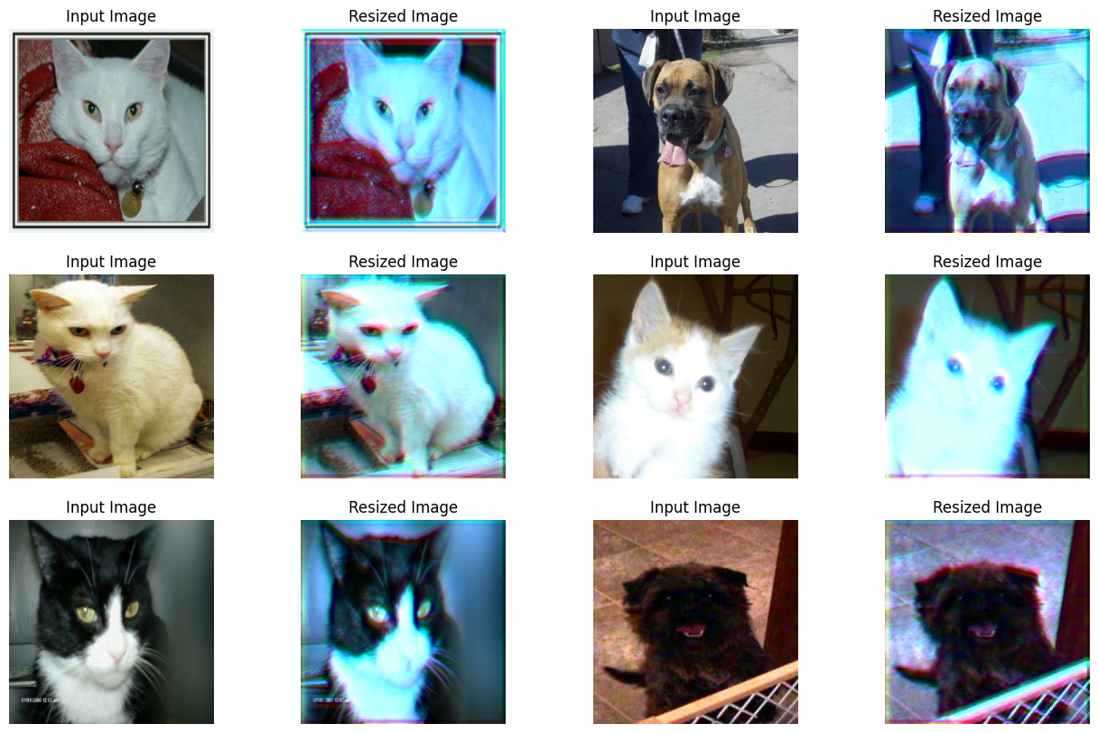
視覺化可學習調整大小模組的輸出
在這裡,我們視覺化經過調整大小的圖像在通過調整大小器的隨機權重後會是什麼樣子。
sample_images, _ = next(iter(train_ds))


plt.figure(figsize=(16, 10))
for i, image in enumerate(sample_images[:6]):
    image = image / 255

    ax = plt.subplot(3, 4, 2 * i + 1)
    plt.title("Input Image")
    plt.imshow(image.numpy().squeeze())
    plt.axis("off")

    ax = plt.subplot(3, 4, 2 * i + 2)
    resized_image = learnable_resizer(image[None, ...])
    plt.title("Resized Image")
    plt.imshow(resized_image.numpy().squeeze())
    plt.axis("off")
Corrupt JPEG data: 65 extraneous bytes before marker 0xd9
WARNING:matplotlib.image:Clipping input data to the valid range for imshow with RGB data ([0..1] for floats or [0..255] for integers).
WARNING:matplotlib.image:Clipping input data to the valid range for imshow with RGB data ([0..1] for floats or [0..255] for integers).
WARNING:matplotlib.image:Clipping input data to the valid range for imshow with RGB data ([0..1] for floats or [0..255] for integers).
WARNING:matplotlib.image:Clipping input data to the valid range for imshow with RGB data ([0..1] for floats or [0..255] for integers).
WARNING:matplotlib.image:Clipping input data to the valid range for imshow with RGB data ([0..1] for floats or [0..255] for integers).
WARNING:matplotlib.image:Clipping input data to the valid range for imshow with RGB data ([0..1] for floats or [0..255] for integers).
模型建構工具
def get_model():
    backbone = keras.applications.DenseNet121(
        weights=None,
        include_top=True,
        classes=2,
        input_shape=((TARGET_SIZE[0], TARGET_SIZE[1], 3)),
    )
    backbone.trainable = True

    inputs = layers.Input((INP_SIZE[0], INP_SIZE[1], 3))
    x = layers.Rescaling(scale=1.0 / 255)(inputs)
    x = learnable_resizer(x)
    outputs = backbone(x)

    return keras.Model(inputs, outputs)
可學習圖像調整大小模組的結構允許與不同的視覺模型進行靈活的整合。
編譯並使用可學習調整大小器訓練我們的模型
model = get_model()
model.compile(
    loss=keras.losses.CategoricalCrossentropy(label_smoothing=0.1),
    optimizer="sgd",
    metrics=["accuracy"],
)
model.fit(train_ds, validation_data=validation_ds, epochs=EPOCHS)
Epoch 1/5

 146/146 ━━━━━━━━━━━━━━━━━━━━ 1790s 12s/step - accuracy: 0.5783 - loss: 0.6877 - val_accuracy: 0.4953 - val_loss: 0.7173

Epoch 2/5

 146/146 ━━━━━━━━━━━━━━━━━━━━ 1738s 12s/step - accuracy: 0.6516 - loss: 0.6436 - val_accuracy: 0.6148 - val_loss: 0.6605

Epoch 3/5

 146/146 ━━━━━━━━━━━━━━━━━━━━ 1730s 12s/step - accuracy: 0.6881 - loss: 0.6185 - val_accuracy: 0.5529 - val_loss: 0.8655

Epoch 4/5

 146/146 ━━━━━━━━━━━━━━━━━━━━ 1725s 12s/step - accuracy: 0.6985 - loss: 0.5980 - val_accuracy: 0.6862 - val_loss: 0.6070

Epoch 5/5

 146/146 ━━━━━━━━━━━━━━━━━━━━ 1722s 12s/step - accuracy: 0.7499 - loss: 0.5595 - val_accuracy: 0.6737 - val_loss: 0.6321

<keras.src.callbacks.history.History at 0x7f126c5440a0>
視覺化已訓練視覺化器的輸出
plt.figure(figsize=(16, 10))
for i, image in enumerate(sample_images[:6]):
    image = image / 255

    ax = plt.subplot(3, 4, 2 * i + 1)
    plt.title("Input Image")
    plt.imshow(image.numpy().squeeze())
    plt.axis("off")

    ax = plt.subplot(3, 4, 2 * i + 2)
    resized_image = learnable_resizer(image[None, ...])
    plt.title("Resized Image")
    plt.imshow(resized_image.numpy().squeeze() / 10)
    plt.axis("off")
WARNING:matplotlib.image:Clipping input data to the valid range for imshow with RGB data ([0..1] for floats or [0..255] for integers).
WARNING:matplotlib.image:Clipping input data to the valid range for imshow with RGB data ([0..1] for floats or [0..255] for integers).
WARNING:matplotlib.image:Clipping input data to the valid range for imshow with RGB data ([0..1] for floats or [0..255] for integers).
WARNING:matplotlib.image:Clipping input data to the valid range for imshow with RGB data ([0..1] for floats or [0..255] for integers).
WARNING:matplotlib.image:Clipping input data to the valid range for imshow with RGB data ([0..1] for floats or [0..255] for integers).
WARNING:matplotlib.image:Clipping input data to the valid range for imshow with RGB data ([0..1] for floats or [0..255] for integers).
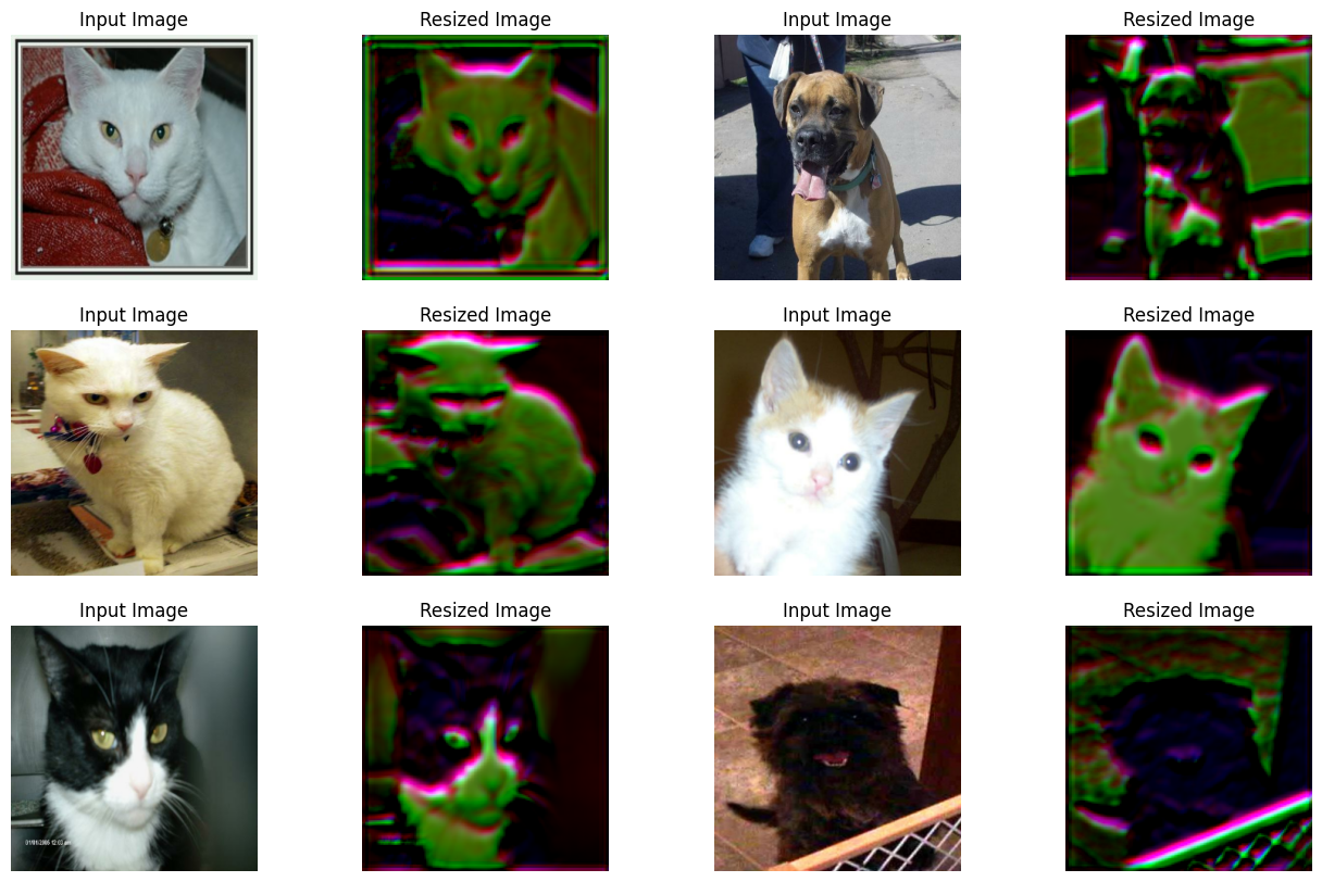
圖表顯示,隨著訓練的進行,影像的視覺效果有所改善。下表顯示了使用調整大小模組相較於使用雙線性插值的優勢。
| 模型 | 參數數量 (百萬) | Top-1 準確度 |
|---|---|---|
| 使用可學習的調整大小器 | 7.051717 | 67.67% |
| 不使用可學習的調整大小器 | 7.039554 | 60.19% |
如需更多詳細資訊,您可以查看此儲存庫。請注意,上述報告的模型是在貓狗資料集的 90% 訓練集上訓練了 10 個 epoch,這與此範例不同。另外,請注意,由於調整大小模組而增加的參數數量非常少。為了確保效能的改進不是由於隨機性,這些模型在訓練時使用了相同的初始隨機權重。
現在,這裡有一個值得探討的問題 - 相較於基準模型,準確度的提高是否僅僅是因為在模型中添加了更多層 (畢竟,調整大小器是一個迷你網路)?
為了證明情況並非如此,作者進行了以下實驗
- 取一個預訓練模型,該模型在某個大小 (例如 224 x 224) 上進行訓練。
- 現在,首先,使用它來推斷調整大小為較低解析度的影像的預測。記錄效能。
- 對於第二個實驗,將調整大小模組插入預訓練模型的頂部,並開始熱啟動訓練。記錄效能。
現在,作者認為使用第二個選項更好,因為它有助於模型學習如何更好地根據給定的解析度調整表示。由於結果純粹是經驗性的,因此進行更多實驗 (例如分析跨通道互動) 會更好。值得注意的是,諸如Squeeze and Excitation (SE) 區塊、Global Context (GC) 區塊之類的元素也會在現有網路中添加一些參數,但它們已知可以幫助網路以系統化的方式處理資訊,以提高整體效能。
注意事項
- 為了在視覺模型內部施加形狀偏差,Geirhos 等人使用自然影像和風格化影像的組合來訓練它們。如果這個可學習的調整大小模組可以達到類似的效果,那將很有趣,因為輸出的結果似乎會丟棄紋理資訊。
- 調整大小模組可以處理任意解析度和長寬比,這對於物件偵測和分割等任務非常重要。
- 還有另一個密切相關的主題,即自適應影像調整大小,它嘗試在訓練期間自適應地調整影像/特徵圖的大小。EfficientV2 使用了這個概念。