用於圖像相似度搜尋的度量學習
作者: Mat Kelcey
建立日期 2020/06/05
上次修改日期 2020/06/09
描述: 在 CIFAR-10 圖像上使用相似度度量學習的範例。

概觀
度量學習旨在訓練模型,使其能夠將輸入嵌入到高維空間中,使得「相似」的輸入(由訓練方案定義)彼此靠近。這些模型一旦經過訓練,就可以為下游系統產生嵌入,其中這種相似性很有用;範例包括作為搜尋的排名訊號,或作為另一個監督問題的預訓練嵌入模型。
有關度量學習的更詳細概觀,請參閱
設定
將 Keras 後端設定為 tensorflow。
import os

os.environ["KERAS_BACKEND"] = "tensorflow"

import random
import matplotlib.pyplot as plt
import numpy as np
import tensorflow as tf
from collections import defaultdict
from PIL import Image
from sklearn.metrics import ConfusionMatrixDisplay
import keras
from keras import layers
資料集
在此範例中,我們將使用 CIFAR-10 資料集。
from keras.datasets import cifar10


(x_train, y_train), (x_test, y_test) = cifar10.load_data()

x_train = x_train.astype("float32") / 255.0
y_train = np.squeeze(y_train)
x_test = x_test.astype("float32") / 255.0
y_test = np.squeeze(y_test)
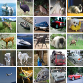
為了了解資料集,我們可以視覺化 25 個隨機範例的網格。
height_width = 32


def show_collage(examples):
    box_size = height_width + 2
    num_rows, num_cols = examples.shape[:2]

    collage = Image.new(
        mode="RGB",
        size=(num_cols * box_size, num_rows * box_size),
        color=(250, 250, 250),
    )
    for row_idx in range(num_rows):
        for col_idx in range(num_cols):
            array = (np.array(examples[row_idx, col_idx]) * 255).astype(np.uint8)
            collage.paste(
                Image.fromarray(array), (col_idx * box_size, row_idx * box_size)
            )

    # Double size for visualisation.
    collage = collage.resize((2 * num_cols * box_size, 2 * num_rows * box_size))
    return collage


# Show a collage of 5x5 random images.
sample_idxs = np.random.randint(0, 50000, size=(5, 5))
examples = x_train[sample_idxs]
show_collage(examples)
度量學習提供的訓練資料並非明確的 (X, y) 配對,而是使用以我們想要表達相似性的方式相關的多個實例。在我們的範例中,我們將使用相同類別的實例來表示相似性;單個訓練實例將不是一個圖像,而是一對相同類別的圖像。在指稱此配對中的圖像時,我們將使用 anchor(隨機選擇的圖像)和 positive(相同類別的另一個隨機選擇的圖像)的常見度量學習名稱。
為了促進這一點,我們需要建立一種查詢形式,該查詢從類別對應到該類別的實例。在產生用於訓練的資料時,我們將從此查詢中取樣。
class_idx_to_train_idxs = defaultdict(list)
for y_train_idx, y in enumerate(y_train):
    class_idx_to_train_idxs[y].append(y_train_idx)

class_idx_to_test_idxs = defaultdict(list)
for y_test_idx, y in enumerate(y_test):
    class_idx_to_test_idxs[y].append(y_test_idx)
在此範例中,我們使用最簡單的訓練方法;一個批次將由跨類別分佈的 (anchor, positive) 配對組成。學習的目標是將 anchor 和 positive 配對拉近,並使其遠離批次中的其他實例。在這種情況下,批次大小將由類別的數量決定;對於 CIFAR-10,此數為 10。
num_classes = 10


class AnchorPositivePairs(keras.utils.Sequence):
    def __init__(self, num_batches):
        super().__init__()
        self.num_batches = num_batches

    def __len__(self):
        return self.num_batches

    def __getitem__(self, _idx):
        x = np.empty((2, num_classes, height_width, height_width, 3), dtype=np.float32)
        for class_idx in range(num_classes):
            examples_for_class = class_idx_to_train_idxs[class_idx]
            anchor_idx = random.choice(examples_for_class)
            positive_idx = random.choice(examples_for_class)
            while positive_idx == anchor_idx:
                positive_idx = random.choice(examples_for_class)
            x[0, class_idx] = x_train[anchor_idx]
            x[1, class_idx] = x_train[positive_idx]
        return x
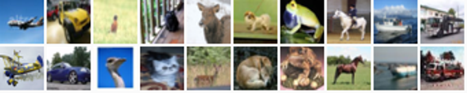
我們可以在另一個拼貼畫中視覺化一個批次。頂行顯示從 10 個類別中隨機選擇的 anchor,底行顯示對應的 10 個 positives。
examples = next(iter(AnchorPositivePairs(num_batches=1)))

show_collage(examples)
嵌入模型
我們定義了一個自訂模型,其中 train_step 首先嵌入 anchors 和 positives,然後使用它們的成對點積作為 softmax 的 logits。
class EmbeddingModel(keras.Model):
    def train_step(self, data):
        # Note: Workaround for open issue, to be removed.
        if isinstance(data, tuple):
            data = data[0]
        anchors, positives = data[0], data[1]

        with tf.GradientTape() as tape:
            # Run both anchors and positives through model.
            anchor_embeddings = self(anchors, training=True)
            positive_embeddings = self(positives, training=True)

            # Calculate cosine similarity between anchors and positives. As they have
            # been normalised this is just the pair wise dot products.
            similarities = keras.ops.einsum(
                "ae,pe->ap", anchor_embeddings, positive_embeddings
            )

            # Since we intend to use these as logits we scale them by a temperature.
            # This value would normally be chosen as a hyper parameter.
            temperature = 0.2
            similarities /= temperature

            # We use these similarities as logits for a softmax. The labels for
            # this call are just the sequence [0, 1, 2, ..., num_classes] since we
            # want the main diagonal values, which correspond to the anchor/positive
            # pairs, to be high. This loss will move embeddings for the
            # anchor/positive pairs together and move all other pairs apart.
            sparse_labels = keras.ops.arange(num_classes)
            loss = self.compute_loss(y=sparse_labels, y_pred=similarities)

        # Calculate gradients and apply via optimizer.
        gradients = tape.gradient(loss, self.trainable_variables)
        self.optimizer.apply_gradients(zip(gradients, self.trainable_variables))

        # Update and return metrics (specifically the one for the loss value).
        for metric in self.metrics:
            # Calling `self.compile` will by default add a [`keras.metrics.Mean`](/api/metrics/metrics_wrappers#mean-class) loss
            if metric.name == "loss":
                metric.update_state(loss)
            else:
                metric.update_state(sparse_labels, similarities)

        return {m.name: m.result() for m in self.metrics}
接下來,我們描述從圖像對應到嵌入的架構。此模型僅包含一系列 2D 卷積,然後是全域池化,以及最後到嵌入空間的線性投影。正如度量學習中常見的那樣,我們將嵌入正規化,以便可以使用簡單的點積來測量相似度。為簡單起見,此模型有意做得較小。
inputs = layers.Input(shape=(height_width, height_width, 3))
x = layers.Conv2D(filters=32, kernel_size=3, strides=2, activation="relu")(inputs)
x = layers.Conv2D(filters=64, kernel_size=3, strides=2, activation="relu")(x)
x = layers.Conv2D(filters=128, kernel_size=3, strides=2, activation="relu")(x)
x = layers.GlobalAveragePooling2D()(x)
embeddings = layers.Dense(units=8, activation=None)(x)
embeddings = layers.UnitNormalization()(embeddings)

model = EmbeddingModel(inputs, embeddings)
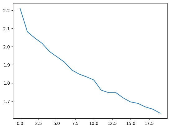
最後,我們執行訓練。在 Google Colab GPU 實例上,這大約需要一分鐘。
model.compile(
    optimizer=keras.optimizers.Adam(learning_rate=1e-3),
    loss=keras.losses.SparseCategoricalCrossentropy(from_logits=True),
)

history = model.fit(AnchorPositivePairs(num_batches=1000), epochs=20)

plt.plot(history.history["loss"])
plt.show()
Epoch 1/20
77/1000 ━[37m━━━━━━━━━━━━━━━━━━━ 1s 2ms/step - loss: 2.2962
WARNING: All log messages before absl::InitializeLog() is called are written to STDERR
I0000 00:00:1700589927.295343 3724442 device_compiler.h:187] Compiled cluster using XLA! This line is logged at most once for the lifetime of the process.
1000/1000 ━━━━━━━━━━━━━━━━━━━━ 6s 2ms/step - loss: 2.2504
Epoch 2/20
1000/1000 ━━━━━━━━━━━━━━━━━━━━ 2s 2ms/step - loss: 2.1068
Epoch 3/20
1000/1000 ━━━━━━━━━━━━━━━━━━━━ 2s 2ms/step - loss: 2.0646
Epoch 4/20
1000/1000 ━━━━━━━━━━━━━━━━━━━━ 2s 2ms/step - loss: 2.0210
Epoch 5/20
1000/1000 ━━━━━━━━━━━━━━━━━━━━ 2s 2ms/step - loss: 1.9857
Epoch 6/20
1000/1000 ━━━━━━━━━━━━━━━━━━━━ 2s 2ms/step - loss: 1.9543
Epoch 7/20
1000/1000 ━━━━━━━━━━━━━━━━━━━━ 2s 2ms/step - loss: 1.9175
Epoch 8/20
1000/1000 ━━━━━━━━━━━━━━━━━━━━ 2s 2ms/step - loss: 1.8740
Epoch 9/20
1000/1000 ━━━━━━━━━━━━━━━━━━━━ 2s 2ms/step - loss: 1.8474
Epoch 10/20
1000/1000 ━━━━━━━━━━━━━━━━━━━━ 2s 2ms/step - loss: 1.8380
Epoch 11/20
1000/1000 ━━━━━━━━━━━━━━━━━━━━ 2s 2ms/step - loss: 1.8146
Epoch 12/20
1000/1000 ━━━━━━━━━━━━━━━━━━━━ 2s 2ms/step - loss: 1.7658
Epoch 13/20
1000/1000 ━━━━━━━━━━━━━━━━━━━━ 2s 2ms/step - loss: 1.7512
Epoch 14/20
1000/1000 ━━━━━━━━━━━━━━━━━━━━ 2s 2ms/step - loss: 1.7671
Epoch 15/20
1000/1000 ━━━━━━━━━━━━━━━━━━━━ 2s 2ms/step - loss: 1.7245
Epoch 16/20
1000/1000 ━━━━━━━━━━━━━━━━━━━━ 2s 2ms/step - loss: 1.7001
Epoch 17/20
1000/1000 ━━━━━━━━━━━━━━━━━━━━ 2s 2ms/step - loss: 1.7099
Epoch 18/20
1000/1000 ━━━━━━━━━━━━━━━━━━━━ 2s 2ms/step - loss: 1.6775
Epoch 19/20
1000/1000 ━━━━━━━━━━━━━━━━━━━━ 2s 2ms/step - loss: 1.6547
Epoch 20/20
1000/1000 ━━━━━━━━━━━━━━━━━━━━ 2s 2ms/step - loss: 1.6356
測試
我們可以將此模型應用於測試集,並考量嵌入空間中的近鄰來檢視此模型的品質。
首先,我們嵌入測試集並計算所有近鄰。回想一下,由於嵌入是單位長度,我們可以透過點積計算餘弦相似度。
near_neighbours_per_example = 10

embeddings = model.predict(x_test)
gram_matrix = np.einsum("ae,be->ab", embeddings, embeddings)
near_neighbours = np.argsort(gram_matrix.T)[:, -(near_neighbours_per_example + 1) :]
313/313 ━━━━━━━━━━━━━━━━━━━━ 1s 3ms/step
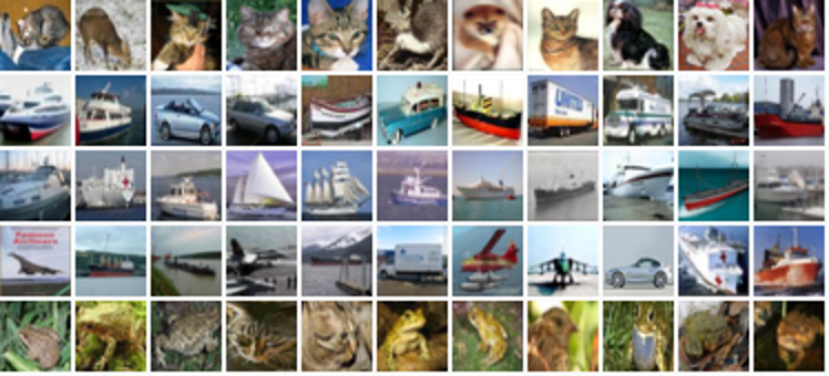
作為這些嵌入的視覺檢查,我們可以為 5 個隨機範例建立近鄰的拼貼畫。下方圖像的第一欄是隨機選取的圖像,接下來的 10 欄按相似度順序顯示最近的鄰居。
num_collage_examples = 5

examples = np.empty(
    (
        num_collage_examples,
        near_neighbours_per_example + 1,
        height_width,
        height_width,
        3,
    ),
    dtype=np.float32,
)
for row_idx in range(num_collage_examples):
    examples[row_idx, 0] = x_test[row_idx]
    anchor_near_neighbours = reversed(near_neighbours[row_idx][:-1])
    for col_idx, nn_idx in enumerate(anchor_near_neighbours):
        examples[row_idx, col_idx + 1] = x_test[nn_idx]

show_collage(examples)
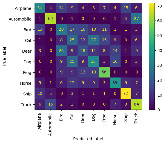
我們還可以透過考量近鄰在混淆矩陣方面的正確性來取得效能的量化檢視。
讓我們從 10 個類別中的每一個取樣 10 個範例,並將它們的近鄰視為一種預測形式;也就是說,範例及其近鄰是否共用相同的類別?
我們觀察到,每個動物類別通常都表現良好,並且最容易與其他動物類別混淆。車輛類別遵循相同的模式。
confusion_matrix = np.zeros((num_classes, num_classes))

# For each class.
for class_idx in range(num_classes):
    # Consider 10 examples.
    example_idxs = class_idx_to_test_idxs[class_idx][:10]
    for y_test_idx in example_idxs:
        # And count the classes of its near neighbours.
        for nn_idx in near_neighbours[y_test_idx][:-1]:
            nn_class_idx = y_test[nn_idx]
            confusion_matrix[class_idx, nn_class_idx] += 1

# Display a confusion matrix.
labels = [
    "Airplane",
    "Automobile",
    "Bird",
    "Cat",
    "Deer",
    "Dog",
    "Frog",
    "Horse",
    "Ship",
    "Truck",
]
disp = ConfusionMatrixDisplay(confusion_matrix=confusion_matrix, display_labels=labels)
disp.plot(include_values=True, cmap="viridis", ax=None, xticks_rotation="vertical")
plt.show()