使用 TensorFlow Similarity 進行影像相似度搜尋的度量學習
作者: Owen Vallis
建立日期 2021/09/30
上次修改日期 2022/02/29
描述: 在 CIFAR-10 影像上使用相似度量學習的範例。

概述
此範例基於 「用於影像相似度搜尋的度量學習」範例。我們的目標是使用相同的資料集,但使用 TensorFlow Similarity 實作模型。
度量學習旨在訓練能夠將輸入嵌入高維空間的模型,以便將「相似」的輸入拉得更近,並將「不相似」的輸入推得更遠。一旦經過訓練,這些模型就可以為下游系統產生嵌入,在這些系統中,這種相似性很有用,例如作為搜尋的排名訊號,或是作為另一個監督問題的預訓練嵌入模型。
如需度量學習的更詳細概述,請參閱
設定
本教學課程將使用 TensorFlow Similarity 程式庫來學習和評估相似度嵌入。TensorFlow Similarity 提供以下元件
- 使訓練對比模型變得簡單快速。
- 更容易確保批次包含成對的範例。
- 能夠評估嵌入的品質。
TensorFlow Similarity 可以透過 pip 輕鬆安裝,如下所示
pip -q install tensorflow_similarity
import random

from matplotlib import pyplot as plt
from mpl_toolkits import axes_grid1
import numpy as np

import tensorflow as tf
from tensorflow import keras

import tensorflow_similarity as tfsim


tfsim.utils.tf_cap_memory()

print("TensorFlow:", tf.__version__)
print("TensorFlow Similarity:", tfsim.__version__)
TensorFlow: 2.7.0
TensorFlow Similarity: 0.15.5
資料集取樣器
在本教學課程中,我們將使用 CIFAR-10 資料集。
為了使相似度模型有效率地學習,每個批次必須包含每個類別的至少 2 個範例。
為了簡化此操作,tf_similarity 提供 Sampler 物件,可讓您設定每個批次的類別數量和每個類別的最小範例數量。
訓練和驗證資料集將使用 TFDatasetMultiShotMemorySampler 物件建立。這會建立一個取樣器,從 TensorFlow Datasets 載入資料集,並產生包含目標類別數量和每個類別目標範例數量的批次。此外,我們可以將取樣器限制為僅產生 class_list 中定義的類別子集,讓我們可以在類別子集上進行訓練,然後測試嵌入如何泛化到看不見的類別。這在處理少樣本學習問題時非常有用。
以下儲存格會建立一個 train_ds 範例,該範例
- 從 TFDS 載入 CIFAR-10 資料集,然後取得
examples_per_class_per_batch。 - 確保取樣器將類別限制為
class_list中定義的類別。 - 確保每個批次包含 10 個不同的類別,每個類別有 8 個範例。
我們也以相同的方式建立驗證資料集,但我們將每個類別的範例總數限制為 100,並且每個批次的每個類別範例數設定為預設值 2。
# This determines the number of classes used during training.
# Here we are using all the classes.
num_known_classes = 10
class_list = random.sample(population=range(10), k=num_known_classes)

classes_per_batch = 10
# Passing multiple examples per class per batch ensures that each example has
# multiple positive pairs. This can be useful when performing triplet mining or
# when using losses like `MultiSimilarityLoss` or `CircleLoss` as these can
# take a weighted mix of all the positive pairs. In general, more examples per
# class will lead to more information for the positive pairs, while more classes
# per batch will provide more varied information in the negative pairs. However,
# the losses compute the pairwise distance between the examples in a batch so
# the upper limit of the batch size is restricted by the memory.
examples_per_class_per_batch = 8

print(
    "Batch size is: "
    f"{min(classes_per_batch, num_known_classes) * examples_per_class_per_batch}"
)

print(" Create Training Data ".center(34, "#"))
train_ds = tfsim.samplers.TFDatasetMultiShotMemorySampler(
    "cifar10",
    classes_per_batch=min(classes_per_batch, num_known_classes),
    splits="train",
    steps_per_epoch=4000,
    examples_per_class_per_batch=examples_per_class_per_batch,
    class_list=class_list,
)

print("\n" + " Create Validation Data ".center(34, "#"))
val_ds = tfsim.samplers.TFDatasetMultiShotMemorySampler(
    "cifar10",
    classes_per_batch=classes_per_batch,
    splits="test",
    total_examples_per_class=100,
)
Batch size is: 80
###### Create Training Data ######

converting train:   0%|          | 0/50000 [00:00<?, ?it/s]
The initial batch size is 80 (10 classes * 8 examples per class) with 0 augmenters

filtering examples:   0%|          | 0/50000 [00:00<?, ?it/s]

selecting classes:   0%|          | 0/10 [00:00<?, ?it/s]

gather examples:   0%|          | 0/50000 [00:00<?, ?it/s]

indexing classes:   0%|          | 0/50000 [00:00<?, ?it/s]
##### Create Validation Data #####

converting test:   0%|          | 0/10000 [00:00<?, ?it/s]
The initial batch size is 20 (10 classes * 2 examples per class) with 0 augmenters

filtering examples:   0%|          | 0/10000 [00:00<?, ?it/s]

selecting classes:   0%|          | 0/10 [00:00<?, ?it/s]

gather examples:   0%|          | 0/1000 [00:00<?, ?it/s]

indexing classes:   0%|          | 0/1000 [00:00<?, ?it/s]
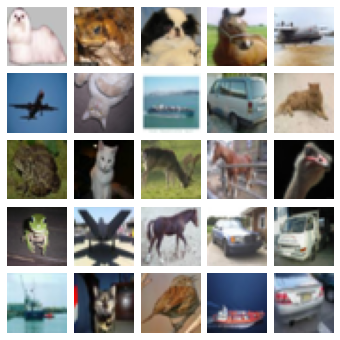
視覺化資料集
取樣器會對資料集進行洗牌,因此我們可以透過繪製前 25 張影像來了解資料集。
取樣器提供 get_slice(begin, size) 方法,可讓我們輕鬆選取範例區塊。
或者,我們可以使用 generate_batch() 方法來產生批次。這可以讓我們檢查批次是否包含預期的類別數量和每個類別的範例數量。
num_cols = num_rows = 5
# Get the first 25 examples.
x_slice, y_slice = train_ds.get_slice(begin=0, size=num_cols * num_rows)

fig = plt.figure(figsize=(6.0, 6.0))
grid = axes_grid1.ImageGrid(fig, 111, nrows_ncols=(num_cols, num_rows), axes_pad=0.1)

for ax, im, label in zip(grid, x_slice, y_slice):
    ax.imshow(im)
    ax.axis("off")
嵌入模型
接下來,我們使用 Keras Functional API 定義 SimilarityModel。該模型是一個標準卷積網路,並新增了一個套用 L2 正規化的 MetricEmbedding 層。當使用 Cosine 距離時,度量嵌入層很有用,因為我們只關心向量之間的角度。
此外,SimilarityModel 還提供了許多輔助方法,用於
- 索引嵌入的範例
- 執行範例查找
- 評估分類結果
- 評估嵌入空間的品質
詳情請參閱 TensorFlow Similarity 文件。
embedding_size = 256

inputs = keras.layers.Input((32, 32, 3))
x = keras.layers.Rescaling(scale=1.0 / 255)(inputs)
x = keras.layers.Conv2D(64, 3, activation="relu")(x)
x = keras.layers.BatchNormalization()(x)
x = keras.layers.Conv2D(128, 3, activation="relu")(x)
x = keras.layers.BatchNormalization()(x)
x = keras.layers.MaxPool2D((4, 4))(x)
x = keras.layers.Conv2D(256, 3, activation="relu")(x)
x = keras.layers.BatchNormalization()(x)
x = keras.layers.Conv2D(256, 3, activation="relu")(x)
x = keras.layers.GlobalMaxPool2D()(x)
outputs = tfsim.layers.MetricEmbedding(embedding_size)(x)

# building model
model = tfsim.models.SimilarityModel(inputs, outputs)
model.summary()
Model: "similarity_model"
_________________________________________________________________
 Layer (type)                Output Shape              Param #
=================================================================
 input_1 (InputLayer)        [(None, 32, 32, 3)]       0

 rescaling (Rescaling)       (None, 32, 32, 3)         0

 conv2d (Conv2D)             (None, 30, 30, 64)        1792

 batch_normalization (BatchN  (None, 30, 30, 64)       256
 ormalization)

 conv2d_1 (Conv2D)           (None, 28, 28, 128)       73856

 batch_normalization_1 (Batc  (None, 28, 28, 128)      512
 hNormalization)

 max_pooling2d (MaxPooling2D  (None, 7, 7, 128)        0
 )

 conv2d_2 (Conv2D)           (None, 5, 5, 256)         295168

 batch_normalization_2 (Batc  (None, 5, 5, 256)        1024
 hNormalization)

 conv2d_3 (Conv2D)           (None, 3, 3, 256)         590080

 global_max_pooling2d (Globa  (None, 256)              0
 lMaxPooling2D)

 metric_embedding (MetricEmb  (None, 256)              65792
 edding)

=================================================================
Total params: 1,028,480
Trainable params: 1,027,584
Non-trainable params: 896
_________________________________________________________________
相似性損失
相似性損失預期批次包含每個類別至少 2 個範例,並從中計算成對正負距離的損失。這裡我們使用 MultiSimilarityLoss()(論文),這是 TensorFlow Similarity 中的幾種損失之一。此損失嘗試使用批次中所有具資訊性的配對,並考量自相似性、正相似性和負相似性。
epochs = 3
learning_rate = 0.002
val_steps = 50

# init similarity loss
loss = tfsim.losses.MultiSimilarityLoss()

# compiling and training
model.compile(
    optimizer=keras.optimizers.Adam(learning_rate), loss=loss, steps_per_execution=10,
)
history = model.fit(
    train_ds, epochs=epochs, validation_data=val_ds, validation_steps=val_steps
)
Distance metric automatically set to cosine use the distance arg to override.
Epoch 1/3

4000/4000 [==============================] - ETA: 0s - loss: 2.2179Warmup complete
4000/4000 [==============================] - 38s 9ms/step - loss: 2.2179 - val_loss: 0.8894
Warmup complete
Epoch 2/3
4000/4000 [==============================] - 34s 9ms/step - loss: 1.9047 - val_loss: 0.8767
Epoch 3/3
4000/4000 [==============================] - 35s 9ms/step - loss: 1.6336 - val_loss: 0.8469
建立索引
現在我們已經訓練好模型,我們可以為範例建立索引。這裡我們將前 200 個驗證範例進行批次索引,方法是將 x 和 y 傳遞到索引中,並將影像儲存在資料參數中。x_index 值會被嵌入,然後新增到索引中以使其可搜尋。y_index 和資料參數是選填的,但允許使用者將中繼資料與嵌入的範例建立關聯。
x_index, y_index = val_ds.get_slice(begin=0, size=200)
model.reset_index()
model.index(x_index, y_index, data=x_index)
[Indexing 200 points]
|-Computing embeddings
|-Storing data points in key value store
|-Adding embeddings to index.
|-Building index.
0%   10   20   30   40   50   60   70   80   90   100%
|----|----|----|----|----|----|----|----|----|----|
***************************************************
校正
建立索引後,我們可以使用比對策略和校正指標來校正距離閾值。
這裡我們在使用 K=1 作為分類器的同時,搜尋最佳 F1 分數。所有小於或等於校正閾值距離的比對都將標示為查詢範例與比對結果相關聯標籤之間的「正向比對」,而所有高於閾值距離的比對都將標示為「負向比對」。
此外,我們還傳入額外的指標以進行計算。輸出中的所有值都是在校正的閾值下計算的。
最後,model.calibrate() 會傳回包含下列項目的 CalibrationResults 物件
"cutpoints":Python 字典,將切點名稱對應到包含與特定距離閾值相關聯的ClassificationMetric值的字典,例如"optimal" : {"acc": 0.90, "f1": 0.92}。"thresholds":Python 字典,將ClassificationMetric名稱對應到一個清單,其中包含在每個距離閾值下計算的指標值,例如{"f1": [0.99, 0.80], "distance": [0.0, 1.0]}。
x_train, y_train = train_ds.get_slice(begin=0, size=1000)
calibration = model.calibrate(
    x_train,
    y_train,
    calibration_metric="f1",
    matcher="match_nearest",
    extra_metrics=["precision", "recall", "binary_accuracy"],
    verbose=1,
)
Performing NN search
Building NN list:   0%|          | 0/1000 [00:00<?, ?it/s]

Evaluating:   0%|          | 0/4 [00:00<?, ?it/s]

computing thresholds:   0%|          | 0/989 [00:00<?, ?it/s]
 name       value    distance    precision    recall    binary_accuracy        f1
-------  -------  ----------  -----------  --------  -----------------  --------
optimal     0.93    0.048435        0.869         1              0.869  0.929909
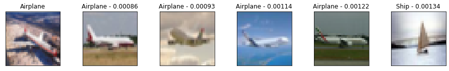
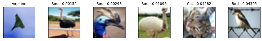
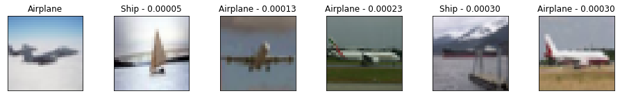
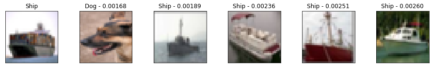
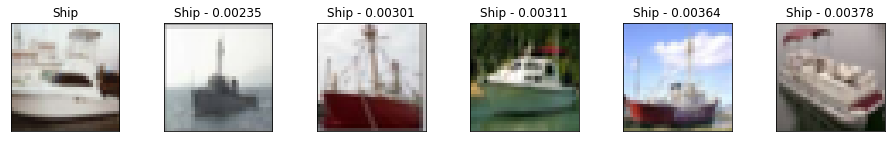
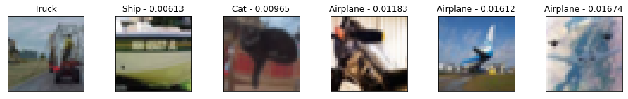
視覺化
單從指標可能難以了解模型品質。另一種輔助方法是手動檢查一組查詢結果,以了解比對品質。
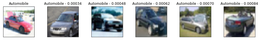
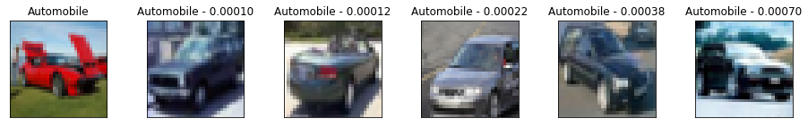
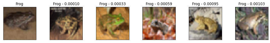
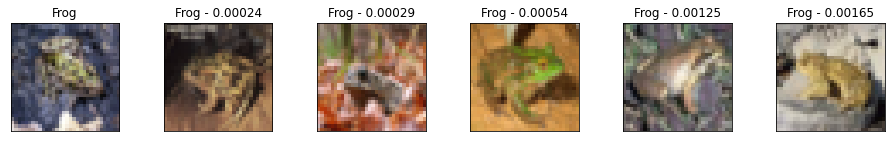
這裡我們取 10 個驗證範例,並將它們與 5 個最接近的鄰居以及與查詢範例的距離一起繪製。查看結果,我們發現雖然它們並不完美,但仍然代表著有意義的相似影像,並且模型能夠找到相似的影像,無論其姿態或影像光照如何。
我們還可以發現模型對某些影像非常有信心,導致查詢和鄰居之間的距離非常小。相反地,當距離變大時,我們在類別標籤中會看到更多錯誤。這就是為什麼校正在比對應用程式中至關重要的原因之一。
num_neighbors = 5
labels = [
    "Airplane",
    "Automobile",
    "Bird",
    "Cat",
    "Deer",
    "Dog",
    "Frog",
    "Horse",
    "Ship",
    "Truck",
    "Unknown",
]
class_mapping = {c_id: c_lbl for c_id, c_lbl in zip(range(11), labels)}

x_display, y_display = val_ds.get_slice(begin=200, size=10)
# lookup nearest neighbors in the index
nns = model.lookup(x_display, k=num_neighbors)

# display
for idx in np.argsort(y_display):
    tfsim.visualization.viz_neigbors_imgs(
        x_display[idx],
        y_display[idx],
        nns[idx],
        class_mapping=class_mapping,
        fig_size=(16, 2),
    )
Performing NN search
Building NN list: 0%| | 0/10 [00:00<?, ?it/s]
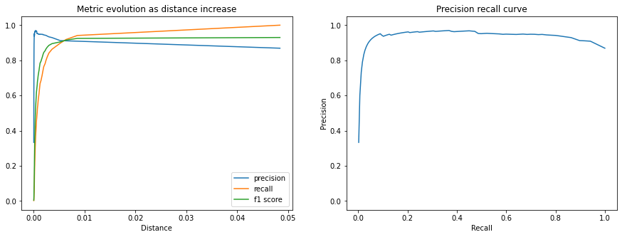
指標
我們還可以繪製 CalibrationResults 中包含的額外指標,以了解比對效能如何隨著距離閾值的增加而變化。
以下圖表顯示精確度、召回率和 F1 分數。我們可以發現,隨著距離增加,比對精確度會降低,但我們接受為正向比對的查詢百分比(召回率)會更快地增長到校正距離閾值。
fig, (ax1, ax2) = plt.subplots(1, 2, figsize=(15, 5))
x = calibration.thresholds["distance"]

ax1.plot(x, calibration.thresholds["precision"], label="precision")
ax1.plot(x, calibration.thresholds["recall"], label="recall")
ax1.plot(x, calibration.thresholds["f1"], label="f1 score")
ax1.legend()
ax1.set_title("Metric evolution as distance increase")
ax1.set_xlabel("Distance")
ax1.set_ylim((-0.05, 1.05))

ax2.plot(calibration.thresholds["recall"], calibration.thresholds["precision"])
ax2.set_title("Precision recall curve")
ax2.set_xlabel("Recall")
ax2.set_ylabel("Precision")
ax2.set_ylim((-0.05, 1.05))
plt.show()
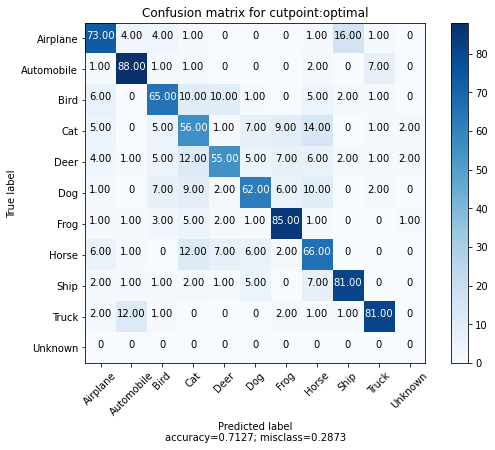
我們還可以為每個類別取 100 個範例,並繪製每個範例及其最接近比對的混淆矩陣。我們還新增一個「額外」的第 10 個類別,表示高於校正距離閾值的比對。
我們可以看到,大多數錯誤發生在動物類別之間,並且在飛機和鳥類之間存在有趣的混淆。此外,我們看到每個類別的 100 個範例中,只有少數範例傳回校正距離閾值外的比對。
cutpoint = "optimal"

# This yields 100 examples for each class.
# We defined this when we created the val_ds sampler.
x_confusion, y_confusion = val_ds.get_slice(0, -1)

matches = model.match(x_confusion, cutpoint=cutpoint, no_match_label=10)
cm = tfsim.visualization.confusion_matrix(
    matches,
    y_confusion,
    labels=labels,
    title="Confusion matrix for cutpoint:%s" % cutpoint,
    normalize=False,
)
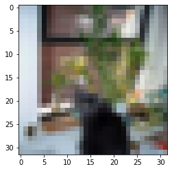
不比對
我們可以繪製校正閾值外的範例,以查看哪些影像未與任何已建立索引的範例比對。
這可能有助於深入了解可能需要建立索引的其他範例,或顯示類別中的異常範例。
idx_no_match = np.where(np.array(matches) == 10)
no_match_queries = x_confusion[idx_no_match]
if len(no_match_queries):
    plt.imshow(no_match_queries[0])
else:
    print("All queries have a match below the distance threshold.")
視覺化叢集
快速了解模型執行品質並了解其缺點的最佳方法之一,是將嵌入投影到 2D 空間中。
這讓我們可以檢查影像叢集,並了解哪些類別纏結在一起。
# Each class in val_ds was restricted to 100 examples.
num_examples_to_clusters = 1000
thumb_size = 96
plot_size = 800
vx, vy = val_ds.get_slice(0, num_examples_to_clusters)

# Uncomment to run the interactive projector.
# tfsim.visualization.projector(
#     model.predict(vx),
#     labels=vy,
#     images=vx,
#     class_mapping=class_mapping,
#     image_size=thumb_size,
#     plot_size=plot_size,
# )