使用雙編碼器的自然語言圖像搜尋
作者: Khalid Salama
建立日期 2021/01/30
上次修改日期 2021/01/30
描述: 實作一個雙編碼器模型,用於檢索符合自然語言查詢的圖像。

簡介
此範例示範如何建構雙編碼器(也稱為雙塔)神經網路模型,以使用自然語言搜尋圖像。該模型受到 Alec Radford 等人提出的 CLIP 方法的啟發。其概念是聯合訓練視覺編碼器和文字編碼器,將圖像及其標題的表示投影到相同的嵌入空間,使得標題嵌入位於其描述的圖像嵌入附近。
此範例需要 TensorFlow 2.4 或更高版本。此外,TensorFlow Hub 和 TensorFlow Text 是 BERT 模型所必需的,而 TensorFlow Addons 是 AdamW 優化器所必需的。可以使用以下命令安裝這些函式庫
pip install -q -U tensorflow-hub tensorflow-text tensorflow-addons
設定
import os
import collections
import json
import numpy as np
import tensorflow as tf
from tensorflow import keras
from tensorflow.keras import layers
import tensorflow_hub as hub
import tensorflow_text as text
import tensorflow_addons as tfa
import matplotlib.pyplot as plt
import matplotlib.image as mpimg
from tqdm import tqdm

# Suppressing tf.hub warnings
tf.get_logger().setLevel("ERROR")
準備資料
我們將使用 MS-COCO 數據集來訓練我們的雙編碼器模型。MS-COCO 包含超過 82,000 張圖像,每張圖像至少有 5 個不同的標題註釋。該數據集通常用於 圖像標題任務,但我們可以重新利用圖像標題對來訓練我們的雙編碼器模型以進行圖像搜尋。
下載並解壓縮資料
首先,讓我們下載數據集,它由兩個壓縮資料夾組成:一個包含圖像,另一個包含相關的圖像標題。請注意,壓縮圖像資料夾的大小為 13GB。
root_dir = "datasets"
annotations_dir = os.path.join(root_dir, "annotations")
images_dir = os.path.join(root_dir, "train2014")
tfrecords_dir = os.path.join(root_dir, "tfrecords")
annotation_file = os.path.join(annotations_dir, "captions_train2014.json")

# Download caption annotation files
if not os.path.exists(annotations_dir):
    annotation_zip = tf.keras.utils.get_file(
        "captions.zip",
        cache_dir=os.path.abspath("."),
        origin="http://images.cocodataset.org/annotations/annotations_trainval2014.zip",
        extract=True,
    )
    os.remove(annotation_zip)

# Download image files
if not os.path.exists(images_dir):
    image_zip = tf.keras.utils.get_file(
        "train2014.zip",
        cache_dir=os.path.abspath("."),
        origin="http://images.cocodataset.org/zips/train2014.zip",
        extract=True,
    )
    os.remove(image_zip)

print("Dataset is downloaded and extracted successfully.")

with open(annotation_file, "r") as f:
    annotations = json.load(f)["annotations"]

image_path_to_caption = collections.defaultdict(list)
for element in annotations:
    caption = f"{element['caption'].lower().rstrip('.')}"
    image_path = images_dir + "/COCO_train2014_" + "%012d.jpg" % (element["image_id"])
    image_path_to_caption[image_path].append(caption)

image_paths = list(image_path_to_caption.keys())
print(f"Number of images: {len(image_paths)}")
Downloading data from http://images.cocodataset.org/annotations/annotations_trainval2014.zip
252878848/252872794 [==============================] - 5s 0us/step
Downloading data from http://images.cocodataset.org/zips/train2014.zip
13510574080/13510573713 [==============================] - 394s 0us/step
Dataset is downloaded and extracted successfully.
Number of images: 82783
處理資料並儲存到 TFRecord 檔案
您可以更改 sample_size 參數來控制將使用多少圖像標題對來訓練雙編碼器模型。在此範例中,我們將 train_size 設定為 30,000 張圖像,約佔數據集的 35%。我們為每張圖像使用 2 個標題,因此產生 60,000 個圖像標題對。訓練集的大小會影響產生的編碼器的品質,但更多範例會導致更長的訓練時間。
train_size = 30000
valid_size = 5000
captions_per_image = 2
images_per_file = 2000

train_image_paths = image_paths[:train_size]
num_train_files = int(np.ceil(train_size / images_per_file))
train_files_prefix = os.path.join(tfrecords_dir, "train")

valid_image_paths = image_paths[-valid_size:]
num_valid_files = int(np.ceil(valid_size / images_per_file))
valid_files_prefix = os.path.join(tfrecords_dir, "valid")

tf.io.gfile.makedirs(tfrecords_dir)


def bytes_feature(value):
    return tf.train.Feature(bytes_list=tf.train.BytesList(value=[value]))


def create_example(image_path, caption):
    feature = {
        "caption": bytes_feature(caption.encode()),
        "raw_image": bytes_feature(tf.io.read_file(image_path).numpy()),
    }
    return tf.train.Example(features=tf.train.Features(feature=feature))


def write_tfrecords(file_name, image_paths):
    caption_list = []
    image_path_list = []
    for image_path in image_paths:
        captions = image_path_to_caption[image_path][:captions_per_image]
        caption_list.extend(captions)
        image_path_list.extend([image_path] * len(captions))

    with tf.io.TFRecordWriter(file_name) as writer:
        for example_idx in range(len(image_path_list)):
            example = create_example(
                image_path_list[example_idx], caption_list[example_idx]
            )
            writer.write(example.SerializeToString())
    return example_idx + 1


def write_data(image_paths, num_files, files_prefix):
    example_counter = 0
    for file_idx in tqdm(range(num_files)):
        file_name = files_prefix + "-%02d.tfrecord" % (file_idx)
        start_idx = images_per_file * file_idx
        end_idx = start_idx + images_per_file
        example_counter += write_tfrecords(file_name, image_paths[start_idx:end_idx])
    return example_counter


train_example_count = write_data(train_image_paths, num_train_files, train_files_prefix)
print(f"{train_example_count} training examples were written to tfrecord files.")

valid_example_count = write_data(valid_image_paths, num_valid_files, valid_files_prefix)
print(f"{valid_example_count} evaluation examples were written to tfrecord files.")
100%|███████████████████████████████████████████████████████████████████████████████████████████████████████████████████████████| 15/15 [03:19<00:00, 13.27s/it]
  0%|                                                                                                                                     | 0/3 [00:00<?, ?it/s]

60000 training examples were written to tfrecord files.

100%|█████████████████████████████████████████████████████████████████████████████████████████████████████████████████████████████| 3/3 [00:33<00:00, 11.07s/it]

10000 evaluation examples were written to tfrecord files.
建立用於訓練和評估的 tf.data.Dataset
feature_description = {
    "caption": tf.io.FixedLenFeature([], tf.string),
    "raw_image": tf.io.FixedLenFeature([], tf.string),
}


def read_example(example):
    features = tf.io.parse_single_example(example, feature_description)
    raw_image = features.pop("raw_image")
    features["image"] = tf.image.resize(
        tf.image.decode_jpeg(raw_image, channels=3), size=(299, 299)
    )
    return features


def get_dataset(file_pattern, batch_size):

    return (
        tf.data.TFRecordDataset(tf.data.Dataset.list_files(file_pattern))
        .map(
            read_example,
            num_parallel_calls=tf.data.AUTOTUNE,
            deterministic=False,
        )
        .shuffle(batch_size * 10)
        .prefetch(buffer_size=tf.data.AUTOTUNE)
        .batch(batch_size)
    )
實作投影頭
投影頭用於將圖像和文字嵌入轉換為具有相同維度的相同嵌入空間。
def project_embeddings(
    embeddings, num_projection_layers, projection_dims, dropout_rate
):
    projected_embeddings = layers.Dense(units=projection_dims)(embeddings)
    for _ in range(num_projection_layers):
        x = tf.nn.gelu(projected_embeddings)
        x = layers.Dense(projection_dims)(x)
        x = layers.Dropout(dropout_rate)(x)
        x = layers.Add()([projected_embeddings, x])
        projected_embeddings = layers.LayerNormalization()(x)
    return projected_embeddings
實作視覺編碼器
在此範例中,我們使用來自 Keras Applications 的 Xception 作為視覺編碼器的基礎。
def create_vision_encoder(
    num_projection_layers, projection_dims, dropout_rate, trainable=False
):
    # Load the pre-trained Xception model to be used as the base encoder.
    xception = keras.applications.Xception(
        include_top=False, weights="imagenet", pooling="avg"
    )
    # Set the trainability of the base encoder.
    for layer in xception.layers:
        layer.trainable = trainable
    # Receive the images as inputs.
    inputs = layers.Input(shape=(299, 299, 3), name="image_input")
    # Preprocess the input image.
    xception_input = tf.keras.applications.xception.preprocess_input(inputs)
    # Generate the embeddings for the images using the xception model.
    embeddings = xception(xception_input)
    # Project the embeddings produced by the model.
    outputs = project_embeddings(
        embeddings, num_projection_layers, projection_dims, dropout_rate
    )
    # Create the vision encoder model.
    return keras.Model(inputs, outputs, name="vision_encoder")
實作文字編碼器
我們使用來自 TensorFlow Hub 的 BERT 作為文字編碼器
def create_text_encoder(
    num_projection_layers, projection_dims, dropout_rate, trainable=False
):
    # Load the BERT preprocessing module.
    preprocess = hub.KerasLayer(
        "https://tfhub.dev/tensorflow/bert_en_uncased_preprocess/2",
        name="text_preprocessing",
    )
    # Load the pre-trained BERT model to be used as the base encoder.
    bert = hub.KerasLayer(
        "https://tfhub.dev/tensorflow/small_bert/bert_en_uncased_L-4_H-512_A-8/1",
        "bert",
    )
    # Set the trainability of the base encoder.
    bert.trainable = trainable
    # Receive the text as inputs.
    inputs = layers.Input(shape=(), dtype=tf.string, name="text_input")
    # Preprocess the text.
    bert_inputs = preprocess(inputs)
    # Generate embeddings for the preprocessed text using the BERT model.
    embeddings = bert(bert_inputs)["pooled_output"]
    # Project the embeddings produced by the model.
    outputs = project_embeddings(
        embeddings, num_projection_layers, projection_dims, dropout_rate
    )
    # Create the text encoder model.
    return keras.Model(inputs, outputs, name="text_encoder")
實作雙編碼器
為了計算損失,我們會計算批次中每個 caption_i 和 images_j 之間的成對點積相似度作為預測值。caption_i 和 image_j 之間的目標相似度計算方式為 (caption_i 和 caption_j 之間的點積相似度) 與 (image_i 和 image_j 之間的點積相似度) 的平均值。然後,我們使用交叉熵來計算目標值和預測值之間的損失。
class DualEncoder(keras.Model):
    def __init__(self, text_encoder, image_encoder, temperature=1.0, **kwargs):
        super().__init__(**kwargs)
        self.text_encoder = text_encoder
        self.image_encoder = image_encoder
        self.temperature = temperature
        self.loss_tracker = keras.metrics.Mean(name="loss")

    @property
    def metrics(self):
        return [self.loss_tracker]

    def call(self, features, training=False):
        # Place each encoder on a separate GPU (if available).
        # TF will fallback on available devices if there are fewer than 2 GPUs.
        with tf.device("/gpu:0"):
            # Get the embeddings for the captions.
            caption_embeddings = text_encoder(features["caption"], training=training)
        with tf.device("/gpu:1"):
            # Get the embeddings for the images.
            image_embeddings = vision_encoder(features["image"], training=training)
        return caption_embeddings, image_embeddings

    def compute_loss(self, caption_embeddings, image_embeddings):
        # logits[i][j] is the dot_similarity(caption_i, image_j).
        logits = (
            tf.matmul(caption_embeddings, image_embeddings, transpose_b=True)
            / self.temperature
        )
        # images_similarity[i][j] is the dot_similarity(image_i, image_j).
        images_similarity = tf.matmul(
            image_embeddings, image_embeddings, transpose_b=True
        )
        # captions_similarity[i][j] is the dot_similarity(caption_i, caption_j).
        captions_similarity = tf.matmul(
            caption_embeddings, caption_embeddings, transpose_b=True
        )
        # targets[i][j] = avarage dot_similarity(caption_i, caption_j) and dot_similarity(image_i, image_j).
        targets = keras.activations.softmax(
            (captions_similarity + images_similarity) / (2 * self.temperature)
        )
        # Compute the loss for the captions using crossentropy
        captions_loss = keras.losses.categorical_crossentropy(
            y_true=targets, y_pred=logits, from_logits=True
        )
        # Compute the loss for the images using crossentropy
        images_loss = keras.losses.categorical_crossentropy(
            y_true=tf.transpose(targets), y_pred=tf.transpose(logits), from_logits=True
        )
        # Return the mean of the loss over the batch.
        return (captions_loss + images_loss) / 2

    def train_step(self, features):
        with tf.GradientTape() as tape:
            # Forward pass
            caption_embeddings, image_embeddings = self(features, training=True)
            loss = self.compute_loss(caption_embeddings, image_embeddings)
        # Backward pass
        gradients = tape.gradient(loss, self.trainable_variables)
        self.optimizer.apply_gradients(zip(gradients, self.trainable_variables))
        # Monitor loss
        self.loss_tracker.update_state(loss)
        return {"loss": self.loss_tracker.result()}

    def test_step(self, features):
        caption_embeddings, image_embeddings = self(features, training=False)
        loss = self.compute_loss(caption_embeddings, image_embeddings)
        self.loss_tracker.update_state(loss)
        return {"loss": self.loss_tracker.result()}
訓練雙編碼器模型
在這個實驗中,我們凍結文本和影像的基礎編碼器,只讓投影頭可訓練。
num_epochs = 5  # In practice, train for at least 30 epochs
batch_size = 256

vision_encoder = create_vision_encoder(
    num_projection_layers=1, projection_dims=256, dropout_rate=0.1
)
text_encoder = create_text_encoder(
    num_projection_layers=1, projection_dims=256, dropout_rate=0.1
)
dual_encoder = DualEncoder(text_encoder, vision_encoder, temperature=0.05)
dual_encoder.compile(
    optimizer=tfa.optimizers.AdamW(learning_rate=0.001, weight_decay=0.001)
)
請注意,使用 60,000 個影像-標題配對的資料,以 256 的批次大小訓練模型,使用 V100 GPU 加速器,每個 epoch 約需 12 分鐘。如果可以使用 2 個 GPU,則每個 epoch 約需 8 分鐘。
print(f"Number of GPUs: {len(tf.config.list_physical_devices('GPU'))}")
print(f"Number of examples (caption-image pairs): {train_example_count}")
print(f"Batch size: {batch_size}")
print(f"Steps per epoch: {int(np.ceil(train_example_count / batch_size))}")
train_dataset = get_dataset(os.path.join(tfrecords_dir, "train-*.tfrecord"), batch_size)
valid_dataset = get_dataset(os.path.join(tfrecords_dir, "valid-*.tfrecord"), batch_size)
# Create a learning rate scheduler callback.
reduce_lr = keras.callbacks.ReduceLROnPlateau(
    monitor="val_loss", factor=0.2, patience=3
)
# Create an early stopping callback.
early_stopping = tf.keras.callbacks.EarlyStopping(
    monitor="val_loss", patience=5, restore_best_weights=True
)
history = dual_encoder.fit(
    train_dataset,
    epochs=num_epochs,
    validation_data=valid_dataset,
    callbacks=[reduce_lr, early_stopping],
)
print("Training completed. Saving vision and text encoders...")
vision_encoder.save("vision_encoder")
text_encoder.save("text_encoder")
print("Models are saved.")
Number of GPUs: 2
Number of examples (caption-image pairs): 60000
Batch size: 256
Steps per epoch: 235
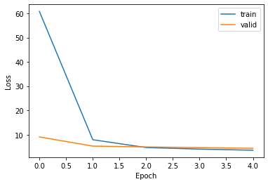
Epoch 1/5
235/235 [==============================] - 573s 2s/step - loss: 60.8318 - val_loss: 9.0531
Epoch 2/5
235/235 [==============================] - 553s 2s/step - loss: 7.8959 - val_loss: 5.2654
Epoch 3/5
235/235 [==============================] - 541s 2s/step - loss: 4.6644 - val_loss: 4.9260
Epoch 4/5
235/235 [==============================] - 538s 2s/step - loss: 4.0188 - val_loss: 4.6312
Epoch 5/5
235/235 [==============================] - 539s 2s/step - loss: 3.5555 - val_loss: 4.3503
Training completed. Saving vision and text encoders...
Models are saved.
繪製訓練損失圖
plt.plot(history.history["loss"])
plt.plot(history.history["val_loss"])
plt.ylabel("Loss")
plt.xlabel("Epoch")
plt.legend(["train", "valid"], loc="upper right")
plt.show()
使用自然語言查詢搜尋圖片
接著,我們可以透過以下步驟檢索與自然語言查詢相對應的圖片:
- 將圖片輸入
vision_encoder來生成圖片的嵌入向量。 - 將自然語言查詢輸入
text_encoder以生成查詢嵌入向量。 - 計算查詢嵌入向量和索引中圖片嵌入向量之間的相似度,以檢索最匹配的索引。
- 查找最匹配圖片的路徑以顯示它們。
請注意,在訓練 dual encoder 之後,只會使用微調後的 vision_encoder 和 text_encoder 模型,而 dual_encoder 模型將會被捨棄。
生成圖片的嵌入向量
我們載入圖片並將它們輸入 vision_encoder 以生成它們的嵌入向量。在大型系統中,此步驟使用平行資料處理框架執行,例如 Apache Spark 或 Apache Beam。生成圖片嵌入向量可能需要數分鐘。
print("Loading vision and text encoders...")
vision_encoder = keras.models.load_model("vision_encoder")
text_encoder = keras.models.load_model("text_encoder")
print("Models are loaded.")


def read_image(image_path):
    image_array = tf.image.decode_jpeg(tf.io.read_file(image_path), channels=3)
    return tf.image.resize(image_array, (299, 299))


print(f"Generating embeddings for {len(image_paths)} images...")
image_embeddings = vision_encoder.predict(
    tf.data.Dataset.from_tensor_slices(image_paths).map(read_image).batch(batch_size),
    verbose=1,
)
print(f"Image embeddings shape: {image_embeddings.shape}.")
Loading vision and text encoders...
Models are loaded.
Generating embeddings for 82783 images...
324/324 [==============================] - 437s 1s/step
Image embeddings shape: (82783, 256).
檢索相關圖片
在這個範例中,我們使用精確匹配,計算輸入查詢嵌入向量和圖片嵌入向量之間的點積相似度,並檢索前 k 個匹配項。但是,在即時使用案例中,為了擴展大量圖片,最好使用近似相似度匹配,使用諸如 ScaNN、Annoy 或 Faiss 之類的框架。
def find_matches(image_embeddings, queries, k=9, normalize=True):
    # Get the embedding for the query.
    query_embedding = text_encoder(tf.convert_to_tensor(queries))
    # Normalize the query and the image embeddings.
    if normalize:
        image_embeddings = tf.math.l2_normalize(image_embeddings, axis=1)
        query_embedding = tf.math.l2_normalize(query_embedding, axis=1)
    # Compute the dot product between the query and the image embeddings.
    dot_similarity = tf.matmul(query_embedding, image_embeddings, transpose_b=True)
    # Retrieve top k indices.
    results = tf.math.top_k(dot_similarity, k).indices.numpy()
    # Return matching image paths.
    return [[image_paths[idx] for idx in indices] for indices in results]
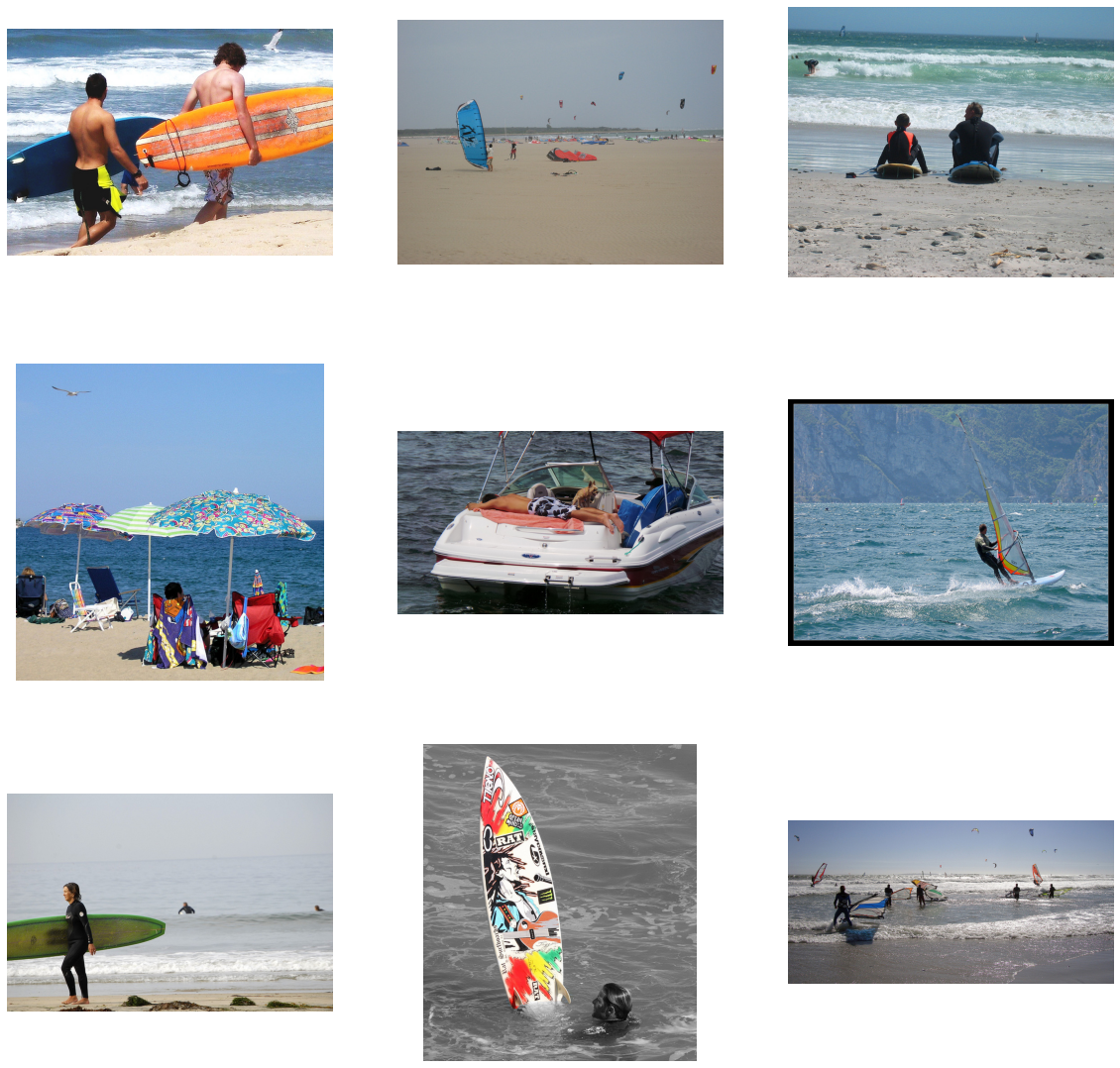
將 query 變數設定為您要搜尋的圖片類型。嘗試一些像是:「一盤健康食物」、「一個戴著帽子的女人走在人行道上」、「一隻鳥坐在水邊」或「野生動物站在田野裡」之類的詞語。
query = "a family standing next to the ocean on a sandy beach with a surf board"
matches = find_matches(image_embeddings, [query], normalize=True)[0]

plt.figure(figsize=(20, 20))
for i in range(9):
    ax = plt.subplot(3, 3, i + 1)
    plt.imshow(mpimg.imread(matches[i]))
    plt.axis("off")
評估檢索品質
為了評估雙編碼器模型,我們使用標題作為查詢。我們使用訓練樣本外的圖片和標題來評估檢索品質,使用前 k 個準確度。如果對於給定的標題,其相關聯的圖片在前 k 個匹配項中被檢索到,則算作真實預測。
def compute_top_k_accuracy(image_paths, k=100):
    hits = 0
    num_batches = int(np.ceil(len(image_paths) / batch_size))
    for idx in tqdm(range(num_batches)):
        start_idx = idx * batch_size
        end_idx = start_idx + batch_size
        current_image_paths = image_paths[start_idx:end_idx]
        queries = [
            image_path_to_caption[image_path][0] for image_path in current_image_paths
        ]
        result = find_matches(image_embeddings, queries, k)
        hits += sum(
            [
                image_path in matches
                for (image_path, matches) in list(zip(current_image_paths, result))
            ]
        )

    return hits / len(image_paths)


print("Scoring training data...")
train_accuracy = compute_top_k_accuracy(train_image_paths)
print(f"Train accuracy: {round(train_accuracy * 100, 3)}%")

print("Scoring evaluation data...")
eval_accuracy = compute_top_k_accuracy(image_paths[train_size:])
print(f"Eval accuracy: {round(eval_accuracy * 100, 3)}%")
  0%|                                                                                                                                   | 0/118 [00:00<?, ?it/s]

Scoring training data...

100%|█████████████████████████████████████████████████████████████████████████████████████████████████████████████████████████| 118/118 [04:12<00:00,  2.14s/it]
  0%|                                                                                                                                   | 0/207 [00:00<?, ?it/s]

Train accuracy: 13.373%
Scoring evaluation data...

100%|█████████████████████████████████████████████████████████████████████████████████████████████████████████████████████████| 207/207 [07:23<00:00,  2.14s/it]

Eval accuracy: 6.235%
最後說明
您可以透過增加訓練樣本的大小、訓練更多 epoch、探索其他影像和文本的基礎編碼器、設定基礎編碼器為可訓練,以及調整超參數,尤其是損失計算中 softmax 的 temperature,來獲得更好的結果。
HuggingFace 上提供的範例
| 已訓練模型 | 演示 |
|---|---|