利用聚合注意力增強卷積網路
作者: Aritra Roy Gosthipaty
建立日期 2022/01/22
上次修改日期 2022/01/22
描述: 建立一個 patch-convnet 架構並視覺化其注意力圖。

簡介
視覺轉換器(Dosovitskiy 等人)已成為卷積神經網路的強大替代方案。視覺轉換器以基於圖塊的方式處理影像。然後,影像資訊會被聚合到一個 CLASS 標記中。此標記會關聯到影像中對於特定分類決策最重要的圖塊。
可以視覺化 CLASS 標記和圖塊之間的交互作用,以幫助解釋分類決策。在學術論文 利用基於注意力的聚合增強卷積網路中,Touvron 等人提出了為卷積網路建立等效視覺化的方法。他們建議將卷積網路的全域平均池化層替換為轉換器層。轉換器的自我注意力層將產生注意力圖,這些注意力圖對應於影像中對於分類決策最受關注的圖塊。
在此範例中,我們最小程度地實作了 利用基於注意力的聚合增強卷積網路 的想法。此範例的主要目標是涵蓋以下想法,並進行少量修改(以調整 CIFAR10 的實作):
- 基於注意力的池化層的簡單設計,使其明確提供不同圖塊的權重(重要性)。
- 卷積網路的新穎架構稱為 PatchConvNet,它偏離了古老的金字塔架構。
設定和匯入
此範例需要 TensorFlow Addons,可以使用以下命令安裝
pip install -U tensorflow-addons
import math
import numpy as np
import tensorflow as tf
from tensorflow import keras
import matplotlib.pyplot as plt
import keras
from keras import layers
from keras import ops
from tensorflow import data as tf_data

# Set seed for reproducibiltiy
SEED = 42
keras.utils.set_random_seed(SEED)
超參數
# DATA
BATCH_SIZE = 128
BUFFER_SIZE = BATCH_SIZE * 2
AUTO = tf_data.AUTOTUNE
INPUT_SHAPE = (32, 32, 3)
NUM_CLASSES = 10  # for CIFAR 10

# AUGMENTATION
IMAGE_SIZE = 48  # We will resize input images to this size.

# ARCHITECTURE
DIMENSIONS = 256
SE_RATIO = 8
TRUNK_DEPTH = 2

# OPTIMIZER
LEARNING_RATE = 1e-3
WEIGHT_DECAY = 1e-4

# PRETRAINING
EPOCHS = 50
載入 CIFAR10 資料集
(x_train, y_train), (x_test, y_test) = keras.datasets.cifar10.load_data()
(x_train, y_train), (x_val, y_val) = (
    (x_train[:40000], y_train[:40000]),
    (x_train[40000:], y_train[40000:]),
)
print(f"Training samples: {len(x_train)}")
print(f"Validation samples: {len(x_val)}")
print(f"Testing samples: {len(x_test)}")

train_ds = tf_data.Dataset.from_tensor_slices((x_train, y_train))
train_ds = train_ds.shuffle(BUFFER_SIZE).batch(BATCH_SIZE).prefetch(AUTO)

val_ds = tf_data.Dataset.from_tensor_slices((x_val, y_val))
val_ds = val_ds.batch(BATCH_SIZE).prefetch(AUTO)

test_ds = tf_data.Dataset.from_tensor_slices((x_test, y_test))
test_ds = test_ds.batch(BATCH_SIZE).prefetch(AUTO)
Downloading data from https://www.cs.toronto.edu/~kriz/cifar-10-python.tar.gz
170500096/170498071 [==============================] - 16s 0us/step
170508288/170498071 [==============================] - 16s 0us/step
Training samples: 40000
Validation samples: 10000
Testing samples: 10000
增強層
def get_preprocessing():
    model = keras.Sequential(
        [
            layers.Rescaling(1 / 255.0),
            layers.Resizing(IMAGE_SIZE, IMAGE_SIZE),
        ],
        name="preprocessing",
    )
    return model


def get_train_augmentation_model():
    model = keras.Sequential(
        [
            layers.Rescaling(1 / 255.0),
            layers.Resizing(INPUT_SHAPE[0] + 20, INPUT_SHAPE[0] + 20),
            layers.RandomCrop(IMAGE_SIZE, IMAGE_SIZE),
            layers.RandomFlip("horizontal"),
        ],
        name="train_data_augmentation",
    )
    return model
卷積幹
模型的幹是一個輕量級的預處理模組,可將影像像素對應到一組向量(圖塊)。
def build_convolutional_stem(dimensions):
    """Build the convolutional stem.

    Args:
        dimensions: The embedding dimension of the patches (d in paper).

    Returs:
        The convolutional stem as a keras seqeuntial
        model.
    """
    config = {
        "kernel_size": (3, 3),
        "strides": (2, 2),
        "activation": ops.gelu,
        "padding": "same",
    }

    convolutional_stem = keras.Sequential(
        [
            layers.Conv2D(filters=dimensions // 2, **config),
            layers.Conv2D(filters=dimensions, **config),
        ],
        name="convolutional_stem",
    )

    return convolutional_stem
卷積主幹
模型的主幹是計算密集度最高的部分。它由 N 個堆疊的殘差卷積區塊組成。
class SqueezeExcite(layers.Layer):
    """Applies squeeze and excitation to input feature maps as seen in
    https://arxiv.org/abs/1709.01507.

    Args:
        ratio: The ratio with which the feature map needs to be reduced in
        the reduction phase.

    Inputs:
        Convolutional features.

    Outputs:
        Attention modified feature maps.
    """

    def __init__(self, ratio, **kwargs):
        super().__init__(**kwargs)
        self.ratio = ratio

    def get_config(self):
        config = super().get_config()
        config.update({"ratio": self.ratio})
        return config

    def build(self, input_shape):
        filters = input_shape[-1]
        self.squeeze = layers.GlobalAveragePooling2D(keepdims=True)
        self.reduction = layers.Dense(
            units=filters // self.ratio,
            activation="relu",
            use_bias=False,
        )
        self.excite = layers.Dense(units=filters, activation="sigmoid", use_bias=False)
        self.multiply = layers.Multiply()

    def call(self, x):
        shortcut = x
        x = self.squeeze(x)
        x = self.reduction(x)
        x = self.excite(x)
        x = self.multiply([shortcut, x])
        return x


class Trunk(layers.Layer):
    """Convolutional residual trunk as in the https://arxiv.org/abs/2112.13692

    Args:
        depth: Number of trunk residual blocks
        dimensions: Dimnesion of the model (denoted by d in the paper)
        ratio: The Squeeze-Excitation ratio

    Inputs:
        Convolutional features extracted from the conv stem.

    Outputs:
        Flattened patches.
    """

    def __init__(self, depth, dimensions, ratio, **kwargs):
        super().__init__(**kwargs)
        self.ratio = ratio
        self.dimensions = dimensions
        self.depth = depth

    def get_config(self):
        config = super().get_config()
        config.update(
            {
                "ratio": self.ratio,
                "dimensions": self.dimensions,
                "depth": self.depth,
            }
        )
        return config

    def build(self, input_shape):
        config = {
            "filters": self.dimensions,
            "activation": ops.gelu,
            "padding": "same",
        }

        trunk_block = [
            layers.LayerNormalization(epsilon=1e-6),
            layers.Conv2D(kernel_size=(1, 1), **config),
            layers.Conv2D(kernel_size=(3, 3), **config),
            SqueezeExcite(ratio=self.ratio),
            layers.Conv2D(kernel_size=(1, 1), filters=self.dimensions, padding="same"),
        ]

        self.trunk_blocks = [keras.Sequential(trunk_block) for _ in range(self.depth)]
        self.add = layers.Add()
        self.flatten_spatial = layers.Reshape((-1, self.dimensions))

    def call(self, x):
        # Remember the input.
        shortcut = x
        for trunk_block in self.trunk_blocks:
            output = trunk_block(x)
            shortcut = self.add([output, shortcut])
            x = shortcut
        # Flatten the patches.
        x = self.flatten_spatial(x)
        return x
注意力池化
卷積主幹的輸出會使用可訓練的查詢類別標記進行關注。產生的注意力圖是影像每個圖塊對於分類決策的權重。
class AttentionPooling(layers.Layer):
    """Applies attention to the patches extracted form the
    trunk with the CLS token.

    Args:
        dimensions: The dimension of the whole architecture.
        num_classes: The number of classes in the dataset.

    Inputs:
        Flattened patches from the trunk.

    Outputs:
        The modifies CLS token.
    """

    def __init__(self, dimensions, num_classes, **kwargs):
        super().__init__(**kwargs)
        self.dimensions = dimensions
        self.num_classes = num_classes
        self.cls = keras.Variable(ops.zeros((1, 1, dimensions)))

    def get_config(self):
        config = super().get_config()
        config.update(
            {
                "dimensions": self.dimensions,
                "num_classes": self.num_classes,
                "cls": self.cls.numpy(),
            }
        )
        return config

    def build(self, input_shape):
        self.attention = layers.MultiHeadAttention(
            num_heads=1,
            key_dim=self.dimensions,
            dropout=0.2,
        )
        self.layer_norm1 = layers.LayerNormalization(epsilon=1e-6)
        self.layer_norm2 = layers.LayerNormalization(epsilon=1e-6)
        self.layer_norm3 = layers.LayerNormalization(epsilon=1e-6)
        self.mlp = keras.Sequential(
            [
                layers.Dense(units=self.dimensions, activation=ops.gelu),
                layers.Dropout(0.2),
                layers.Dense(units=self.dimensions, activation=ops.gelu),
            ]
        )
        self.dense = layers.Dense(units=self.num_classes)
        self.flatten = layers.Flatten()

    def call(self, x):
        batch_size = ops.shape(x)[0]
        # Expand the class token batch number of times.
        class_token = ops.repeat(self.cls, repeats=batch_size, axis=0)
        # Concat the input with the trainable class token.
        x = ops.concatenate([class_token, x], axis=1)
        # Apply attention to x.
        x = self.layer_norm1(x)
        x, viz_weights = self.attention(
            query=x[:, 0:1], key=x, value=x, return_attention_scores=True
        )
        class_token = class_token + x
        class_token = self.layer_norm2(class_token)
        class_token = self.flatten(class_token)
        class_token = self.layer_norm3(class_token)
        class_token = class_token + self.mlp(class_token)
        # Build the logits
        logits = self.dense(class_token)
        return logits, ops.squeeze(viz_weights)[..., 1:]
圖塊卷積網路
圖塊卷積網路如下圖所示。
 |
|---|
| 來源 |
架構中的所有模組都在前面的章節中建立完成。在本節中,我們將把所有不同的模組堆疊在一起。
class PatchConvNet(keras.Model):
    def __init__(
        self,
        stem,
        trunk,
        attention_pooling,
        preprocessing_model,
        train_augmentation_model,
        **kwargs,
    ):
        super().__init__(**kwargs)
        self.stem = stem
        self.trunk = trunk
        self.attention_pooling = attention_pooling
        self.train_augmentation_model = train_augmentation_model
        self.preprocessing_model = preprocessing_model

    def get_config(self):
        config = super().get_config()
        config.update(
            {
                "stem": self.stem,
                "trunk": self.trunk,
                "attention_pooling": self.attention_pooling,
                "train_augmentation_model": self.train_augmentation_model,
                "preprocessing_model": self.preprocessing_model,
            }
        )
        return config

    def _calculate_loss(self, inputs, test=False):
        images, labels = inputs
        # Augment the input images.
        if test:
            augmented_images = self.preprocessing_model(images)
        else:
            augmented_images = self.train_augmentation_model(images)
        # Pass through the stem.
        x = self.stem(augmented_images)
        # Pass through the trunk.
        x = self.trunk(x)
        # Pass through the attention pooling block.
        logits, _ = self.attention_pooling(x)
        # Compute the total loss.
        total_loss = self.compiled_loss(labels, logits)
        return total_loss, logits

    def train_step(self, inputs):
        with tf.GradientTape() as tape:
            total_loss, logits = self._calculate_loss(inputs)
        # Apply gradients.
        train_vars = [
            self.stem.trainable_variables,
            self.trunk.trainable_variables,
            self.attention_pooling.trainable_variables,
        ]
        grads = tape.gradient(total_loss, train_vars)
        trainable_variable_list = []
        for grad, var in zip(grads, train_vars):
            for g, v in zip(grad, var):
                trainable_variable_list.append((g, v))
        self.optimizer.apply_gradients(trainable_variable_list)
        # Report progress.
        _, labels = inputs
        self.compiled_metrics.update_state(labels, logits)
        return {m.name: m.result() for m in self.metrics}

    def test_step(self, inputs):
        total_loss, logits = self._calculate_loss(inputs, test=True)
        # Report progress.
        _, labels = inputs
        self.compiled_metrics.update_state(labels, logits)
        return {m.name: m.result() for m in self.metrics}

    def call(self, images):
        # Augment the input images.
        augmented_images = self.preprocessing_model(images)
        # Pass through the stem.
        x = self.stem(augmented_images)
        # Pass through the trunk.
        x = self.trunk(x)
        # Pass through the attention pooling block.
        logits, viz_weights = self.attention_pooling(x)
        return logits, viz_weights
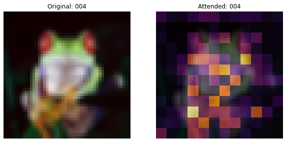
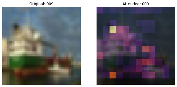
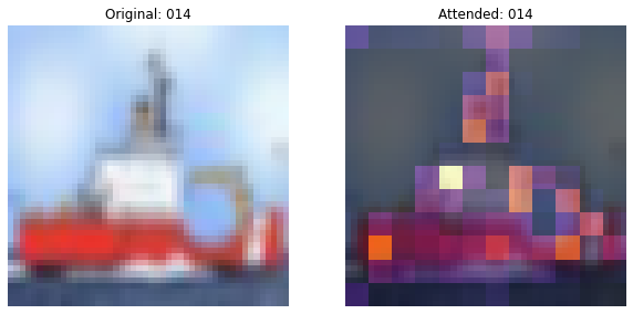
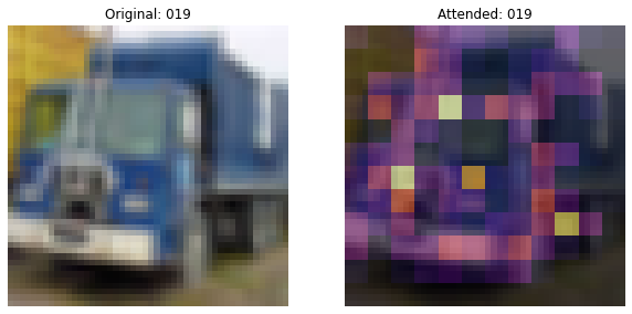
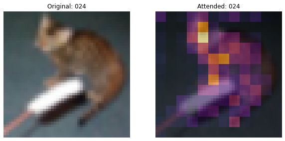
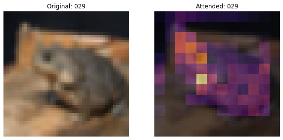
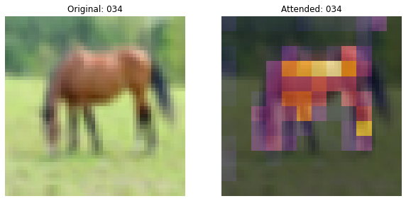
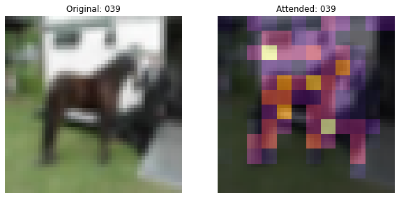
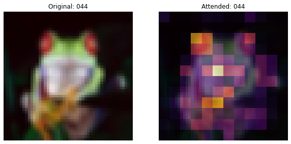
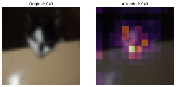
回調函數 (Callbacks)
此回調函數將繪製圖像,並將注意力地圖疊加在圖像上。
# Taking a batch of test inputs to measure model's progress.
test_images, test_labels = next(iter(test_ds))


class TrainMonitor(keras.callbacks.Callback):
    def __init__(self, epoch_interval=None):
        self.epoch_interval = epoch_interval

    def on_epoch_end(self, epoch, logs=None):
        if self.epoch_interval and epoch % self.epoch_interval == 4:
            test_augmented_images = self.model.preprocessing_model(test_images)
            # Pass through the stem.
            test_x = self.model.stem(test_augmented_images)
            # Pass through the trunk.
            test_x = self.model.trunk(test_x)
            # Pass through the attention pooling block.
            _, test_viz_weights = self.model.attention_pooling(test_x)
            # Reshape the vizualization weights
            num_patches = ops.shape(test_viz_weights)[-1]
            height = width = int(math.sqrt(num_patches))
            test_viz_weights = layers.Reshape((height, width))(test_viz_weights)
            # Take a random image and its attention weights.
            index = np.random.randint(low=0, high=ops.shape(test_augmented_images)[0])
            selected_image = test_augmented_images[index]
            selected_weight = test_viz_weights[index]
            # Plot the images and the overlayed attention map.
            fig, ax = plt.subplots(nrows=1, ncols=2, figsize=(10, 5))
            ax[0].imshow(selected_image)
            ax[0].set_title(f"Original: {epoch:03d}")
            ax[0].axis("off")
            img = ax[1].imshow(selected_image)
            ax[1].imshow(
                selected_weight, cmap="inferno", alpha=0.6, extent=img.get_extent()
            )
            ax[1].set_title(f"Attended: {epoch:03d}")
            ax[1].axis("off")
            plt.axis("off")
            plt.show()
            plt.close()
學習率排程 (Learning rate schedule)
class WarmUpCosine(keras.optimizers.schedules.LearningRateSchedule):
    def __init__(
        self, learning_rate_base, total_steps, warmup_learning_rate, warmup_steps
    ):
        super().__init__()
        self.learning_rate_base = learning_rate_base
        self.total_steps = total_steps
        self.warmup_learning_rate = warmup_learning_rate
        self.warmup_steps = warmup_steps
        self.pi = np.pi

    def __call__(self, step):
        if self.total_steps < self.warmup_steps:
            raise ValueError("Total_steps must be larger or equal to warmup_steps.")
        cos_annealed_lr = ops.cos(
            self.pi
            * (ops.cast(step, "float32") - self.warmup_steps)
            / float(self.total_steps - self.warmup_steps)
        )
        learning_rate = 0.5 * self.learning_rate_base * (1 + cos_annealed_lr)
        if self.warmup_steps > 0:
            if self.learning_rate_base < self.warmup_learning_rate:
                raise ValueError(
                    "Learning_rate_base must be larger or equal to "
                    "warmup_learning_rate."
                )
            slope = (
                self.learning_rate_base - self.warmup_learning_rate
            ) / self.warmup_steps
            warmup_rate = slope * ops.cast(step, "float32") + self.warmup_learning_rate
            learning_rate = ops.where(
                step < self.warmup_steps, warmup_rate, learning_rate
            )
        return ops.where(
            step > self.total_steps,
            0.0,
            learning_rate,
        )


total_steps = int((len(x_train) / BATCH_SIZE) * EPOCHS)
warmup_epoch_percentage = 0.15
warmup_steps = int(total_steps * warmup_epoch_percentage)
scheduled_lrs = WarmUpCosine(
    learning_rate_base=LEARNING_RATE,
    total_steps=total_steps,
    warmup_learning_rate=0.0,
    warmup_steps=warmup_steps,
)
訓練 (Training)
我們建立模型、編譯它並進行訓練。
train_augmentation_model = get_train_augmentation_model()
preprocessing_model = get_preprocessing()
conv_stem = build_convolutional_stem(dimensions=DIMENSIONS)
conv_trunk = Trunk(depth=TRUNK_DEPTH, dimensions=DIMENSIONS, ratio=SE_RATIO)
attention_pooling = AttentionPooling(dimensions=DIMENSIONS, num_classes=NUM_CLASSES)

patch_conv_net = PatchConvNet(
    stem=conv_stem,
    trunk=conv_trunk,
    attention_pooling=attention_pooling,
    train_augmentation_model=train_augmentation_model,
    preprocessing_model=preprocessing_model,
)

# Assemble the callbacks.
train_callbacks = [TrainMonitor(epoch_interval=5)]
# Get the optimizer.
optimizer = keras.optimizers.AdamW(
    learning_rate=scheduled_lrs, weight_decay=WEIGHT_DECAY
)
# Compile and pretrain the model.
patch_conv_net.compile(
    optimizer=optimizer,
    loss=keras.losses.SparseCategoricalCrossentropy(from_logits=True),
    metrics=[
        keras.metrics.SparseCategoricalAccuracy(name="accuracy"),
        keras.metrics.SparseTopKCategoricalAccuracy(5, name="top-5-accuracy"),
    ],
)
history = patch_conv_net.fit(
    train_ds,
    epochs=EPOCHS,
    validation_data=val_ds,
    callbacks=train_callbacks,
)

# Evaluate the model with the test dataset.
loss, acc_top1, acc_top5 = patch_conv_net.evaluate(test_ds)
print(f"Loss: {loss:0.2f}")
print(f"Top 1 test accuracy: {acc_top1*100:0.2f}%")
print(f"Top 5 test accuracy: {acc_top5*100:0.2f}%")
Epoch 1/50
313/313 [==============================] - 14s 27ms/step - loss: 1.9639 - accuracy: 0.2635 - top-5-accuracy: 0.7792 - val_loss: 1.7219 - val_accuracy: 0.3778 - val_top-5-accuracy: 0.8514
Epoch 2/50
313/313 [==============================] - 8s 26ms/step - loss: 1.5475 - accuracy: 0.4214 - top-5-accuracy: 0.9099 - val_loss: 1.4351 - val_accuracy: 0.4592 - val_top-5-accuracy: 0.9298
Epoch 3/50
313/313 [==============================] - 8s 25ms/step - loss: 1.3328 - accuracy: 0.5135 - top-5-accuracy: 0.9368 - val_loss: 1.3763 - val_accuracy: 0.5077 - val_top-5-accuracy: 0.9268
Epoch 4/50
313/313 [==============================] - 8s 25ms/step - loss: 1.1653 - accuracy: 0.5807 - top-5-accuracy: 0.9554 - val_loss: 1.0892 - val_accuracy: 0.6146 - val_top-5-accuracy: 0.9560
Epoch 5/50
313/313 [==============================] - ETA: 0s - loss: 1.0235 - accuracy: 0.6345 - top-5-accuracy: 0.9660
313/313 [==============================] - 8s 25ms/step - loss: 1.0235 - accuracy: 0.6345 - top-5-accuracy: 0.9660 - val_loss: 1.0085 - val_accuracy: 0.6424 - val_top-5-accuracy: 0.9640
Epoch 6/50
313/313 [==============================] - 8s 25ms/step - loss: 0.9190 - accuracy: 0.6729 - top-5-accuracy: 0.9741 - val_loss: 0.9066 - val_accuracy: 0.6850 - val_top-5-accuracy: 0.9751
Epoch 7/50
313/313 [==============================] - 8s 25ms/step - loss: 0.8331 - accuracy: 0.7056 - top-5-accuracy: 0.9783 - val_loss: 0.8844 - val_accuracy: 0.6903 - val_top-5-accuracy: 0.9779
Epoch 8/50
313/313 [==============================] - 8s 25ms/step - loss: 0.7526 - accuracy: 0.7376 - top-5-accuracy: 0.9823 - val_loss: 0.8200 - val_accuracy: 0.7114 - val_top-5-accuracy: 0.9793
Epoch 9/50
313/313 [==============================] - 8s 25ms/step - loss: 0.6853 - accuracy: 0.7636 - top-5-accuracy: 0.9856 - val_loss: 0.7216 - val_accuracy: 0.7584 - val_top-5-accuracy: 0.9823
Epoch 10/50
313/313 [==============================] - ETA: 0s - loss: 0.6260 - accuracy: 0.7849 - top-5-accuracy: 0.9877
313/313 [==============================] - 8s 25ms/step - loss: 0.6260 - accuracy: 0.7849 - top-5-accuracy: 0.9877 - val_loss: 0.6985 - val_accuracy: 0.7624 - val_top-5-accuracy: 0.9847
Epoch 11/50
313/313 [==============================] - 8s 25ms/step - loss: 0.5877 - accuracy: 0.7978 - top-5-accuracy: 0.9897 - val_loss: 0.7357 - val_accuracy: 0.7595 - val_top-5-accuracy: 0.9816
Epoch 12/50
313/313 [==============================] - 8s 25ms/step - loss: 0.5615 - accuracy: 0.8066 - top-5-accuracy: 0.9905 - val_loss: 0.6554 - val_accuracy: 0.7806 - val_top-5-accuracy: 0.9841
Epoch 13/50
313/313 [==============================] - 8s 25ms/step - loss: 0.5287 - accuracy: 0.8174 - top-5-accuracy: 0.9915 - val_loss: 0.5867 - val_accuracy: 0.8051 - val_top-5-accuracy: 0.9869
Epoch 14/50
313/313 [==============================] - 8s 25ms/step - loss: 0.4976 - accuracy: 0.8286 - top-5-accuracy: 0.9921 - val_loss: 0.5707 - val_accuracy: 0.8047 - val_top-5-accuracy: 0.9899
Epoch 15/50
313/313 [==============================] - ETA: 0s - loss: 0.4735 - accuracy: 0.8348 - top-5-accuracy: 0.9939
313/313 [==============================] - 8s 25ms/step - loss: 0.4735 - accuracy: 0.8348 - top-5-accuracy: 0.9939 - val_loss: 0.5945 - val_accuracy: 0.8040 - val_top-5-accuracy: 0.9883
Epoch 16/50
313/313 [==============================] - 8s 25ms/step - loss: 0.4660 - accuracy: 0.8364 - top-5-accuracy: 0.9936 - val_loss: 0.5629 - val_accuracy: 0.8125 - val_top-5-accuracy: 0.9906
Epoch 17/50
313/313 [==============================] - 8s 25ms/step - loss: 0.4416 - accuracy: 0.8462 - top-5-accuracy: 0.9946 - val_loss: 0.5747 - val_accuracy: 0.8013 - val_top-5-accuracy: 0.9888
Epoch 18/50
313/313 [==============================] - 8s 25ms/step - loss: 0.4175 - accuracy: 0.8560 - top-5-accuracy: 0.9949 - val_loss: 0.5672 - val_accuracy: 0.8088 - val_top-5-accuracy: 0.9903
Epoch 19/50
313/313 [==============================] - 8s 25ms/step - loss: 0.3912 - accuracy: 0.8650 - top-5-accuracy: 0.9957 - val_loss: 0.5454 - val_accuracy: 0.8136 - val_top-5-accuracy: 0.9907
Epoch 20/50
311/313 [============================>.] - ETA: 0s - loss: 0.3800 - accuracy: 0.8676 - top-5-accuracy: 0.9956
313/313 [==============================] - 8s 25ms/step - loss: 0.3801 - accuracy: 0.8676 - top-5-accuracy: 0.9956 - val_loss: 0.5274 - val_accuracy: 0.8222 - val_top-5-accuracy: 0.9915
Epoch 21/50
313/313 [==============================] - 8s 25ms/step - loss: 0.3641 - accuracy: 0.8734 - top-5-accuracy: 0.9962 - val_loss: 0.5032 - val_accuracy: 0.8315 - val_top-5-accuracy: 0.9921
Epoch 22/50
313/313 [==============================] - 8s 25ms/step - loss: 0.3474 - accuracy: 0.8805 - top-5-accuracy: 0.9970 - val_loss: 0.5251 - val_accuracy: 0.8302 - val_top-5-accuracy: 0.9917
Epoch 23/50
313/313 [==============================] - 8s 25ms/step - loss: 0.3327 - accuracy: 0.8833 - top-5-accuracy: 0.9976 - val_loss: 0.5158 - val_accuracy: 0.8321 - val_top-5-accuracy: 0.9903
Epoch 24/50
313/313 [==============================] - 8s 25ms/step - loss: 0.3158 - accuracy: 0.8897 - top-5-accuracy: 0.9977 - val_loss: 0.5098 - val_accuracy: 0.8355 - val_top-5-accuracy: 0.9912
Epoch 25/50
312/313 [============================>.] - ETA: 0s - loss: 0.2985 - accuracy: 0.8976 - top-5-accuracy: 0.9976
313/313 [==============================] - 8s 25ms/step - loss: 0.2986 - accuracy: 0.8976 - top-5-accuracy: 0.9976 - val_loss: 0.5302 - val_accuracy: 0.8276 - val_top-5-accuracy: 0.9922
Epoch 26/50
313/313 [==============================] - 8s 25ms/step - loss: 0.2819 - accuracy: 0.9021 - top-5-accuracy: 0.9977 - val_loss: 0.5130 - val_accuracy: 0.8358 - val_top-5-accuracy: 0.9923
Epoch 27/50
313/313 [==============================] - 8s 25ms/step - loss: 0.2696 - accuracy: 0.9065 - top-5-accuracy: 0.9983 - val_loss: 0.5096 - val_accuracy: 0.8389 - val_top-5-accuracy: 0.9926
Epoch 28/50
313/313 [==============================] - 8s 25ms/step - loss: 0.2526 - accuracy: 0.9115 - top-5-accuracy: 0.9983 - val_loss: 0.4988 - val_accuracy: 0.8403 - val_top-5-accuracy: 0.9921
Epoch 29/50
313/313 [==============================] - 8s 25ms/step - loss: 0.2322 - accuracy: 0.9190 - top-5-accuracy: 0.9987 - val_loss: 0.5234 - val_accuracy: 0.8395 - val_top-5-accuracy: 0.9915
Epoch 30/50
313/313 [==============================] - ETA: 0s - loss: 0.2180 - accuracy: 0.9235 - top-5-accuracy: 0.9988
313/313 [==============================] - 8s 26ms/step - loss: 0.2180 - accuracy: 0.9235 - top-5-accuracy: 0.9988 - val_loss: 0.5175 - val_accuracy: 0.8407 - val_top-5-accuracy: 0.9925
Epoch 31/50
313/313 [==============================] - 8s 25ms/step - loss: 0.2108 - accuracy: 0.9267 - top-5-accuracy: 0.9990 - val_loss: 0.5046 - val_accuracy: 0.8476 - val_top-5-accuracy: 0.9937
Epoch 32/50
313/313 [==============================] - 8s 25ms/step - loss: 0.1929 - accuracy: 0.9337 - top-5-accuracy: 0.9991 - val_loss: 0.5096 - val_accuracy: 0.8516 - val_top-5-accuracy: 0.9914
Epoch 33/50
313/313 [==============================] - 8s 25ms/step - loss: 0.1787 - accuracy: 0.9370 - top-5-accuracy: 0.9992 - val_loss: 0.4963 - val_accuracy: 0.8541 - val_top-5-accuracy: 0.9917
Epoch 34/50
313/313 [==============================] - 8s 25ms/step - loss: 0.1653 - accuracy: 0.9428 - top-5-accuracy: 0.9994 - val_loss: 0.5092 - val_accuracy: 0.8547 - val_top-5-accuracy: 0.9921
Epoch 35/50
313/313 [==============================] - ETA: 0s - loss: 0.1544 - accuracy: 0.9464 - top-5-accuracy: 0.9995
313/313 [==============================] - 7s 24ms/step - loss: 0.1544 - accuracy: 0.9464 - top-5-accuracy: 0.9995 - val_loss: 0.5137 - val_accuracy: 0.8513 - val_top-5-accuracy: 0.9928
Epoch 36/50
313/313 [==============================] - 8s 25ms/step - loss: 0.1418 - accuracy: 0.9507 - top-5-accuracy: 0.9997 - val_loss: 0.5267 - val_accuracy: 0.8560 - val_top-5-accuracy: 0.9913
Epoch 37/50
313/313 [==============================] - 8s 25ms/step - loss: 0.1259 - accuracy: 0.9561 - top-5-accuracy: 0.9997 - val_loss: 0.5283 - val_accuracy: 0.8584 - val_top-5-accuracy: 0.9923
Epoch 38/50
313/313 [==============================] - 8s 25ms/step - loss: 0.1166 - accuracy: 0.9599 - top-5-accuracy: 0.9997 - val_loss: 0.5541 - val_accuracy: 0.8549 - val_top-5-accuracy: 0.9919
Epoch 39/50
313/313 [==============================] - 8s 25ms/step - loss: 0.1111 - accuracy: 0.9624 - top-5-accuracy: 0.9997 - val_loss: 0.5543 - val_accuracy: 0.8575 - val_top-5-accuracy: 0.9917
Epoch 40/50
312/313 [============================>.] - ETA: 0s - loss: 0.1017 - accuracy: 0.9653 - top-5-accuracy: 0.9997
313/313 [==============================] - 8s 25ms/step - loss: 0.1016 - accuracy: 0.9653 - top-5-accuracy: 0.9997 - val_loss: 0.5357 - val_accuracy: 0.8614 - val_top-5-accuracy: 0.9923
Epoch 41/50
313/313 [==============================] - 8s 25ms/step - loss: 0.0925 - accuracy: 0.9687 - top-5-accuracy: 0.9998 - val_loss: 0.5248 - val_accuracy: 0.8615 - val_top-5-accuracy: 0.9924
Epoch 42/50
313/313 [==============================] - 8s 25ms/step - loss: 0.0848 - accuracy: 0.9726 - top-5-accuracy: 0.9997 - val_loss: 0.5182 - val_accuracy: 0.8654 - val_top-5-accuracy: 0.9939
Epoch 43/50
313/313 [==============================] - 8s 25ms/step - loss: 0.0823 - accuracy: 0.9724 - top-5-accuracy: 0.9999 - val_loss: 0.5010 - val_accuracy: 0.8679 - val_top-5-accuracy: 0.9931
Epoch 44/50
313/313 [==============================] - 8s 25ms/step - loss: 0.0762 - accuracy: 0.9752 - top-5-accuracy: 0.9998 - val_loss: 0.5088 - val_accuracy: 0.8686 - val_top-5-accuracy: 0.9939
Epoch 45/50
312/313 [============================>.] - ETA: 0s - loss: 0.0752 - accuracy: 0.9763 - top-5-accuracy: 0.9999
313/313 [==============================] - 8s 26ms/step - loss: 0.0752 - accuracy: 0.9764 - top-5-accuracy: 0.9999 - val_loss: 0.4844 - val_accuracy: 0.8679 - val_top-5-accuracy: 0.9938
Epoch 46/50
313/313 [==============================] - 8s 25ms/step - loss: 0.0789 - accuracy: 0.9745 - top-5-accuracy: 0.9997 - val_loss: 0.4774 - val_accuracy: 0.8702 - val_top-5-accuracy: 0.9937
Epoch 47/50
313/313 [==============================] - 8s 25ms/step - loss: 0.0866 - accuracy: 0.9726 - top-5-accuracy: 0.9998 - val_loss: 0.4644 - val_accuracy: 0.8666 - val_top-5-accuracy: 0.9936
Epoch 48/50
313/313 [==============================] - 8s 25ms/step - loss: 0.1000 - accuracy: 0.9697 - top-5-accuracy: 0.9999 - val_loss: 0.4471 - val_accuracy: 0.8636 - val_top-5-accuracy: 0.9933
Epoch 49/50
313/313 [==============================] - 8s 25ms/step - loss: 0.1315 - accuracy: 0.9592 - top-5-accuracy: 0.9997 - val_loss: 0.4411 - val_accuracy: 0.8603 - val_top-5-accuracy: 0.9926
Epoch 50/50
313/313 [==============================] - ETA: 0s - loss: 0.1828 - accuracy: 0.9447 - top-5-accuracy: 0.9995
313/313 [==============================] - 8s 25ms/step - loss: 0.1828 - accuracy: 0.9447 - top-5-accuracy: 0.9995 - val_loss: 0.4614 - val_accuracy: 0.8480 - val_top-5-accuracy: 0.9920
79/79 [==============================] - 1s 8ms/step - loss: 0.4696 - accuracy: 0.8459 - top-5-accuracy: 0.9921
Loss: 0.47
Top 1 test accuracy: 84.59%
Top 5 test accuracy: 99.21%
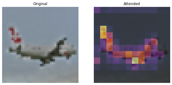
推論 (Inference)
在這裡,我們使用訓練好的模型來繪製注意力地圖。
def plot_attention(image):
    """Plots the attention map on top of the image.

    Args:
        image: A numpy image of arbitrary size.
    """
    # Resize the image to a (32, 32) dim.
    image = ops.image.resize(image, (32, 32))
    image = image[np.newaxis, ...]
    test_augmented_images = patch_conv_net.preprocessing_model(image)
    # Pass through the stem.
    test_x = patch_conv_net.stem(test_augmented_images)
    # Pass through the trunk.
    test_x = patch_conv_net.trunk(test_x)
    # Pass through the attention pooling block.
    _, test_viz_weights = patch_conv_net.attention_pooling(test_x)
    test_viz_weights = test_viz_weights[np.newaxis, ...]
    # Reshape the vizualization weights.
    num_patches = ops.shape(test_viz_weights)[-1]
    height = width = int(math.sqrt(num_patches))
    test_viz_weights = layers.Reshape((height, width))(test_viz_weights)
    selected_image = test_augmented_images[0]
    selected_weight = test_viz_weights[0]
    # Plot the images.
    fig, ax = plt.subplots(nrows=1, ncols=2, figsize=(10, 5))
    ax[0].imshow(selected_image)
    ax[0].set_title(f"Original")
    ax[0].axis("off")
    img = ax[1].imshow(selected_image)
    ax[1].imshow(selected_weight, cmap="inferno", alpha=0.6, extent=img.get_extent())
    ax[1].set_title(f"Attended")
    ax[1].axis("off")
    plt.axis("off")
    plt.show()
    plt.close()


url = "http://farm9.staticflickr.com/8017/7140384795_385b1f48df_z.jpg"
image_name = keras.utils.get_file(fname="image.jpg", origin=url)
image = keras.utils.load_img(image_name)
image = keras.utils.img_to_array(image)
plot_attention(image)
結論 (Conclusions)
對應於可訓練的 CLASS token 和圖像區塊的注意力地圖有助於解釋分類決策。還應該注意到,注意力地圖會逐漸變得更好。在初始訓練階段,注意力分散在各處,而在後期階段,它會更集中於圖像的物件上。
非金字塔卷積網路達到了約 84-85% 的 top-1 測試準確度。
我要感謝 JarvisLabs.ai 為這個專案提供 GPU 額度。