使用 PointNet 進行點雲分割
作者: Soumik Rakshit, Sayak Paul
建立日期 2020/10/23
最後修改日期 2020/10/24
描述: 基於 PointNet 的點雲分割模型實作。

簡介
「點雲」是一種用於儲存幾何形狀資料的重要資料結構。由於其不規則的格式,通常在深度學習應用中使用之前,會將其轉換為規則的 3D 体素網格或圖像集合,這一步會使資料變得不必要地大。PointNet 模型系列透過直接使用點雲解決了這個問題,同時尊重點資料的排列不變性屬性。PointNet 模型系列為應用程式提供了一個簡單、統一的架構,範圍從物件分類、零件分割到場景語義解析。
在此範例中,我們展示了用於形狀分割的 PointNet 架構實作。
參考資料
匯入
import os
import json
import random
import numpy as np
import pandas as pd
from tqdm import tqdm
from glob import glob

import tensorflow as tf  # For tf.data
import keras
from keras import layers

import matplotlib.pyplot as plt
下載資料集
ShapeNet 資料集是一項持續的努力,旨在建立一個具有豐富註解的大規模 3D 形狀資料集。ShapeNetCore 是完整 ShapeNet 資料集的子集,具有乾淨的單個 3D 模型和手動驗證的類別和對齊註解。它涵蓋 55 個常見的物件類別,約有 51,300 個獨特的 3D 模型。
在此範例中,我們使用 PASCAL 3D+ 的 12 個物件類別之一,作為 ShapenetCore 資料集的一部分。
dataset_url = "https://git.io/JiY4i"

dataset_path = keras.utils.get_file(
    fname="shapenet.zip",
    origin=dataset_url,
    cache_subdir="datasets",
    hash_algorithm="auto",
    extract=True,
    archive_format="auto",
    cache_dir="datasets",
)
載入資料集
我們解析資料集元數據,以便輕鬆地將模型類別對應到它們各自的目錄,並將分割類別對應到顏色,以進行視覺化。
with open("/tmp/.keras/datasets/PartAnnotation/metadata.json") as json_file:
    metadata = json.load(json_file)

print(metadata)
{'Airplane': {'directory': '02691156', 'lables': ['wing', 'body', 'tail', 'engine'], 'colors': ['blue', 'green', 'red', 'pink']}, 'Bag': {'directory': '02773838', 'lables': ['handle', 'body'], 'colors': ['blue', 'green']}, 'Cap': {'directory': '02954340', 'lables': ['panels', 'peak'], 'colors': ['blue', 'green']}, 'Car': {'directory': '02958343', 'lables': ['wheel', 'hood', 'roof'], 'colors': ['blue', 'green', 'red']}, 'Chair': {'directory': '03001627', 'lables': ['leg', 'arm', 'back', 'seat'], 'colors': ['blue', 'green', 'red', 'pink']}, 'Earphone': {'directory': '03261776', 'lables': ['earphone', 'headband'], 'colors': ['blue', 'green']}, 'Guitar': {'directory': '03467517', 'lables': ['head', 'body', 'neck'], 'colors': ['blue', 'green', 'red']}, 'Knife': {'directory': '03624134', 'lables': ['handle', 'blade'], 'colors': ['blue', 'green']}, 'Lamp': {'directory': '03636649', 'lables': ['canopy', 'lampshade', 'base'], 'colors': ['blue', 'green', 'red']}, 'Laptop': {'directory': '03642806', 'lables': ['keyboard'], 'colors': ['blue']}, 'Motorbike': {'directory': '03790512', 'lables': ['wheel', 'handle', 'gas_tank', 'light', 'seat'], 'colors': ['blue', 'green', 'red', 'pink', 'yellow']}, 'Mug': {'directory': '03797390', 'lables': ['handle'], 'colors': ['blue']}, 'Pistol': {'directory': '03948459', 'lables': ['trigger_and_guard', 'handle', 'barrel'], 'colors': ['blue', 'green', 'red']}, 'Rocket': {'directory': '04099429', 'lables': ['nose', 'body', 'fin'], 'colors': ['blue', 'green', 'red']}, 'Skateboard': {'directory': '04225987', 'lables': ['wheel', 'deck'], 'colors': ['blue', 'green']}, 'Table': {'directory': '04379243', 'lables': ['leg', 'top'], 'colors': ['blue', 'green']}}
在此範例中,我們訓練 PointNet 來分割Airplane模型的零件。
points_dir = "/tmp/.keras/datasets/PartAnnotation/{}/points".format(
    metadata["Airplane"]["directory"]
)
labels_dir = "/tmp/.keras/datasets/PartAnnotation/{}/points_label".format(
    metadata["Airplane"]["directory"]
)
LABELS = metadata["Airplane"]["lables"]
COLORS = metadata["Airplane"]["colors"]

VAL_SPLIT = 0.2
NUM_SAMPLE_POINTS = 1024
BATCH_SIZE = 32
EPOCHS = 60
INITIAL_LR = 1e-3
建構資料集
我們從飛機點雲及其標籤產生以下記憶體中的資料結構
point_clouds是一個np.array物件清單,以 x、y 和 z 座標的形式表示點雲資料。軸 0 代表點雲中的點數,而軸 1 代表座標。all_labels是一個清單,表示每個座標的標籤為字串(主要用於視覺化目的)。test_point_clouds的格式與point_clouds相同,但不具有對應的點雲標籤。all_labels是一個np.array物件清單,表示每個座標的點雲標籤,對應於point_clouds清單。point_cloud_labels是一個np.array物件清單,表示每個座標的點雲標籤,以 one-hot 編碼的形式表示,對應於point_clouds清單。
point_clouds, test_point_clouds = [], []
point_cloud_labels, all_labels = [], []

points_files = glob(os.path.join(points_dir, "*.pts"))
for point_file in tqdm(points_files):
    point_cloud = np.loadtxt(point_file)
    if point_cloud.shape[0] < NUM_SAMPLE_POINTS:
        continue

    # Get the file-id of the current point cloud for parsing its
    # labels.
    file_id = point_file.split("/")[-1].split(".")[0]
    label_data, num_labels = {}, 0
    for label in LABELS:
        label_file = os.path.join(labels_dir, label, file_id + ".seg")
        if os.path.exists(label_file):
            label_data[label] = np.loadtxt(label_file).astype("float32")
            num_labels = len(label_data[label])

    # Point clouds having labels will be our training samples.
    try:
        label_map = ["none"] * num_labels
        for label in LABELS:
            for i, data in enumerate(label_data[label]):
                label_map[i] = label if data == 1 else label_map[i]
        label_data = [
            LABELS.index(label) if label != "none" else len(LABELS)
            for label in label_map
        ]
        # Apply one-hot encoding to the dense label representation.
        label_data = keras.utils.to_categorical(label_data, num_classes=len(LABELS) + 1)

        point_clouds.append(point_cloud)
        point_cloud_labels.append(label_data)
        all_labels.append(label_map)
    except KeyError:
        test_point_clouds.append(point_cloud)
100%|██████████████████████████████████████████████████████████████████████| 4045/4045 [01:30<00:00, 44.54it/s]
接下來,我們看看剛才產生的記憶體陣列中的一些樣本
for _ in range(5):
    i = random.randint(0, len(point_clouds) - 1)
    print(f"point_clouds[{i}].shape:", point_clouds[0].shape)
    print(f"point_cloud_labels[{i}].shape:", point_cloud_labels[0].shape)
    for j in range(5):
        print(
            f"all_labels[{i}][{j}]:",
            all_labels[i][j],
            f"\tpoint_cloud_labels[{i}][{j}]:",
            point_cloud_labels[i][j],
            "\n",
        )
point_clouds[333].shape: (2571, 3)
point_cloud_labels[333].shape: (2571, 5)
all_labels[333][0]: tail    point_cloud_labels[333][0]: [0. 0. 1. 0. 0.]
all_labels[333][1]: wing point_cloud_labels[333][1]: [1. 0. 0. 0. 0.]
all_labels[333][2]: tail point_cloud_labels[333][2]: [0. 0. 1. 0. 0.]
all_labels[333][3]: engine point_cloud_labels[333][3]: [0. 0. 0. 1. 0.]
all_labels[333][4]: wing point_cloud_labels[333][4]: [1. 0. 0. 0. 0.]
point_clouds[3273].shape: (2571, 3)
point_cloud_labels[3273].shape: (2571, 5)
all_labels[3273][0]: body   point_cloud_labels[3273][0]: [0. 1. 0. 0. 0.]
all_labels[3273][1]: body point_cloud_labels[3273][1]: [0. 1. 0. 0. 0.]
all_labels[3273][2]: tail point_cloud_labels[3273][2]: [0. 0. 1. 0. 0.]
all_labels[3273][3]: wing point_cloud_labels[3273][3]: [1. 0. 0. 0. 0.]
all_labels[3273][4]: wing point_cloud_labels[3273][4]: [1. 0. 0. 0. 0.]
point_clouds[929].shape: (2571, 3)
point_cloud_labels[929].shape: (2571, 5)
all_labels[929][0]: body    point_cloud_labels[929][0]: [0. 1. 0. 0. 0.]
all_labels[929][1]: tail point_cloud_labels[929][1]: [0. 0. 1. 0. 0.]
all_labels[929][2]: wing point_cloud_labels[929][2]: [1. 0. 0. 0. 0.]
all_labels[929][3]: tail point_cloud_labels[929][3]: [0. 0. 1. 0. 0.]
all_labels[929][4]: body point_cloud_labels[929][4]: [0. 1. 0. 0. 0.]
point_clouds[496].shape: (2571, 3)
point_cloud_labels[496].shape: (2571, 5)
all_labels[496][0]: body    point_cloud_labels[496][0]: [0. 1. 0. 0. 0.]
all_labels[496][1]: body point_cloud_labels[496][1]: [0. 1. 0. 0. 0.]
all_labels[496][2]: body point_cloud_labels[496][2]: [0. 1. 0. 0. 0.]
all_labels[496][3]: wing point_cloud_labels[496][3]: [1. 0. 0. 0. 0.]
all_labels[496][4]: body point_cloud_labels[496][4]: [0. 1. 0. 0. 0.]
point_clouds[3508].shape: (2571, 3)
point_cloud_labels[3508].shape: (2571, 5)
all_labels[3508][0]: body   point_cloud_labels[3508][0]: [0. 1. 0. 0. 0.]
all_labels[3508][1]: body point_cloud_labels[3508][1]: [0. 1. 0. 0. 0.]
all_labels[3508][2]: body point_cloud_labels[3508][2]: [0. 1. 0. 0. 0.]
all_labels[3508][3]: body point_cloud_labels[3508][3]: [0. 1. 0. 0. 0.]
all_labels[3508][4]: body point_cloud_labels[3508][4]: [0. 1. 0. 0. 0.]
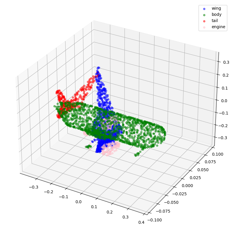
現在,讓我們將一些點雲及其標籤視覺化。
def visualize_data(point_cloud, labels):
    df = pd.DataFrame(
        data={
            "x": point_cloud[:, 0],
            "y": point_cloud[:, 1],
            "z": point_cloud[:, 2],
            "label": labels,
        }
    )
    fig = plt.figure(figsize=(15, 10))
    ax = plt.axes(projection="3d")
    for index, label in enumerate(LABELS):
        c_df = df[df["label"] == label]
        try:
            ax.scatter(
                c_df["x"], c_df["y"], c_df["z"], label=label, alpha=0.5, c=COLORS[index]
            )
        except IndexError:
            pass
    ax.legend()
    plt.show()


visualize_data(point_clouds[0], all_labels[0])
visualize_data(point_clouds[300], all_labels[300])
預處理
請注意,我們已載入的所有點雲都包含可變數量的點,這使得我們難以將它們批次處理在一起。為了克服這個問題,我們從每個點雲中隨機採樣固定數量的點。我們還對點雲進行正規化,以使資料具有尺度不變性。
for index in tqdm(range(len(point_clouds))):
    current_point_cloud = point_clouds[index]
    current_label_cloud = point_cloud_labels[index]
    current_labels = all_labels[index]
    num_points = len(current_point_cloud)
    # Randomly sampling respective indices.
    sampled_indices = random.sample(list(range(num_points)), NUM_SAMPLE_POINTS)
    # Sampling points corresponding to sampled indices.
    sampled_point_cloud = np.array([current_point_cloud[i] for i in sampled_indices])
    # Sampling corresponding one-hot encoded labels.
    sampled_label_cloud = np.array([current_label_cloud[i] for i in sampled_indices])
    # Sampling corresponding labels for visualization.
    sampled_labels = np.array([current_labels[i] for i in sampled_indices])
    # Normalizing sampled point cloud.
    norm_point_cloud = sampled_point_cloud - np.mean(sampled_point_cloud, axis=0)
    norm_point_cloud /= np.max(np.linalg.norm(norm_point_cloud, axis=1))
    point_clouds[index] = norm_point_cloud
    point_cloud_labels[index] = sampled_label_cloud
    all_labels[index] = sampled_labels
100%|█████████████████████████████████████████████████████████████████████| 3694/3694 [00:08<00:00, 446.45it/s]
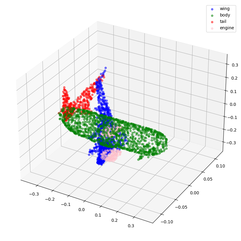
讓我們將採樣和正規化的點雲及其對應的標籤視覺化。
visualize_data(point_clouds[0], all_labels[0])
visualize_data(point_clouds[300], all_labels[300])

建立 TensorFlow 資料集
我們為訓練和驗證資料建立 tf.data.Dataset 物件。我們還透過對訓練點雲應用隨機抖動來增強它們。
def load_data(point_cloud_batch, label_cloud_batch):
    point_cloud_batch.set_shape([NUM_SAMPLE_POINTS, 3])
    label_cloud_batch.set_shape([NUM_SAMPLE_POINTS, len(LABELS) + 1])
    return point_cloud_batch, label_cloud_batch


def augment(point_cloud_batch, label_cloud_batch):
    noise = tf.random.uniform(
        tf.shape(label_cloud_batch), -0.001, 0.001, dtype=tf.float64
    )
    point_cloud_batch += noise[:, :, :3]
    return point_cloud_batch, label_cloud_batch


def generate_dataset(point_clouds, label_clouds, is_training=True):
    dataset = tf.data.Dataset.from_tensor_slices((point_clouds, label_clouds))
    dataset = dataset.shuffle(BATCH_SIZE * 100) if is_training else dataset
    dataset = dataset.map(load_data, num_parallel_calls=tf.data.AUTOTUNE)
    dataset = dataset.batch(batch_size=BATCH_SIZE)
    dataset = (
        dataset.map(augment, num_parallel_calls=tf.data.AUTOTUNE)
        if is_training
        else dataset
    )
    return dataset


split_index = int(len(point_clouds) * (1 - VAL_SPLIT))
train_point_clouds = point_clouds[:split_index]
train_label_cloud = point_cloud_labels[:split_index]
total_training_examples = len(train_point_clouds)

val_point_clouds = point_clouds[split_index:]
val_label_cloud = point_cloud_labels[split_index:]

print("Num train point clouds:", len(train_point_clouds))
print("Num train point cloud labels:", len(train_label_cloud))
print("Num val point clouds:", len(val_point_clouds))
print("Num val point cloud labels:", len(val_label_cloud))

train_dataset = generate_dataset(train_point_clouds, train_label_cloud)
val_dataset = generate_dataset(val_point_clouds, val_label_cloud, is_training=False)

print("Train Dataset:", train_dataset)
print("Validation Dataset:", val_dataset)
Num train point clouds: 2955
Num train point cloud labels: 2955
Num val point clouds: 739
Num val point cloud labels: 739
Train Dataset: <_ParallelMapDataset element_spec=(TensorSpec(shape=(None, 1024, 3), dtype=tf.float64, name=None), TensorSpec(shape=(None, 1024, 5), dtype=tf.float64, name=None))>
Validation Dataset: <_BatchDataset element_spec=(TensorSpec(shape=(None, 1024, 3), dtype=tf.float64, name=None), TensorSpec(shape=(None, 1024, 5), dtype=tf.float64, name=None))>
PointNet 模型
下圖描述了 PointNet 模型系列的內部結構

鑑於 PointNet 旨在將無序集合的座標作為其輸入資料使用,其架構需要符合點雲資料的以下特性
排列不變性
鑑於點雲資料的非結構化性質,由 n 個點組成的掃描具有 n! 種排列方式。後續的資料處理必須對不同的表示形式保持不變。為了使 PointNet 對輸入排列保持不變,一旦 n 個輸入點對應到更高維度的空間,我們就會使用對稱函數(例如最大池化)。結果是全域特徵向量,旨在捕獲 n 個輸入點的聚合簽名。全域特徵向量與局部點特徵一起用於分割。

轉換不變性
如果物體經過某些轉換,例如平移或縮放,分割輸出應該保持不變。對於給定的輸入點雲,我們會應用適當的剛性或仿射轉換來實現姿態正規化。因為每個 n 個輸入點都表示為一個向量,並且獨立地映射到嵌入空間,所以應用幾何轉換僅相當於將每個點與轉換矩陣相乘。這受到空間轉換網路概念的啟發。
構成 T-Net 的操作是受到 PointNet 的更高層次架構的啟發。MLP(或全連接層)用於將輸入點獨立且相同地映射到更高維度的空間;最大池化用於編碼全域特徵向量,然後使用全連接層來降低其維度。最後,最終全連接層中與輸入相關的特徵與全域可訓練的權重和偏差相結合,產生一個 3x3 的轉換矩陣。

點互動
相鄰點之間的互動通常攜帶有用的資訊(即,不應將單個點孤立看待)。雖然分類只需要使用全域特徵,但分割必須能夠利用局部點特徵以及全域點特徵。
注意:本節中呈現的圖形取自原始論文。
現在我們了解了構成 PointNet 模型的各個部分,我們可以開始實作該模型。我們先實作基本區塊,即卷積區塊和多層感知器區塊。
def conv_block(x, filters, name):
    x = layers.Conv1D(filters, kernel_size=1, padding="valid", name=f"{name}_conv")(x)
    x = layers.BatchNormalization(name=f"{name}_batch_norm")(x)
    return layers.Activation("relu", name=f"{name}_relu")(x)


def mlp_block(x, filters, name):
    x = layers.Dense(filters, name=f"{name}_dense")(x)
    x = layers.BatchNormalization(name=f"{name}_batch_norm")(x)
    return layers.Activation("relu", name=f"{name}_relu")(x)
我們實作一個正規化器(取自這個範例)以在特徵空間中強制正交性。這是為了確保轉換後特徵的幅度不會變化太大。
class OrthogonalRegularizer(keras.regularizers.Regularizer):
    """Reference: https://keras.dev.org.tw/examples/vision/pointnet/#build-a-model"""

    def __init__(self, num_features, l2reg=0.001):
        self.num_features = num_features
        self.l2reg = l2reg
        self.identity = keras.ops.eye(num_features)

    def __call__(self, x):
        x = keras.ops.reshape(x, (-1, self.num_features, self.num_features))
        xxt = keras.ops.tensordot(x, x, axes=(2, 2))
        xxt = keras.ops.reshape(xxt, (-1, self.num_features, self.num_features))
        return keras.ops.sum(self.l2reg * keras.ops.square(xxt - self.identity))

    def get_config(self):
        config = super().get_config()
        config.update({"num_features": self.num_features, "l2reg_strength": self.l2reg})
        return config
下一個部分是我們先前解釋過的轉換網路。
def transformation_net(inputs, num_features, name):
    """
    Reference: https://keras.dev.org.tw/examples/vision/pointnet/#build-a-model.

    The `filters` values come from the original paper:
    https://arxiv.org/abs/1612.00593.
    """
    x = conv_block(inputs, filters=64, name=f"{name}_1")
    x = conv_block(x, filters=128, name=f"{name}_2")
    x = conv_block(x, filters=1024, name=f"{name}_3")
    x = layers.GlobalMaxPooling1D()(x)
    x = mlp_block(x, filters=512, name=f"{name}_1_1")
    x = mlp_block(x, filters=256, name=f"{name}_2_1")
    return layers.Dense(
        num_features * num_features,
        kernel_initializer="zeros",
        bias_initializer=keras.initializers.Constant(np.eye(num_features).flatten()),
        activity_regularizer=OrthogonalRegularizer(num_features),
        name=f"{name}_final",
    )(x)


def transformation_block(inputs, num_features, name):
    transformed_features = transformation_net(inputs, num_features, name=name)
    transformed_features = layers.Reshape((num_features, num_features))(
        transformed_features
    )
    return layers.Dot(axes=(2, 1), name=f"{name}_mm")([inputs, transformed_features])
最後,我們將以上區塊組合在一起並實作分割模型。
def get_shape_segmentation_model(num_points, num_classes):
    input_points = keras.Input(shape=(None, 3))

    # PointNet Classification Network.
    transformed_inputs = transformation_block(
        input_points, num_features=3, name="input_transformation_block"
    )
    features_64 = conv_block(transformed_inputs, filters=64, name="features_64")
    features_128_1 = conv_block(features_64, filters=128, name="features_128_1")
    features_128_2 = conv_block(features_128_1, filters=128, name="features_128_2")
    transformed_features = transformation_block(
        features_128_2, num_features=128, name="transformed_features"
    )
    features_512 = conv_block(transformed_features, filters=512, name="features_512")
    features_2048 = conv_block(features_512, filters=2048, name="pre_maxpool_block")
    global_features = layers.MaxPool1D(pool_size=num_points, name="global_features")(
        features_2048
    )
    global_features = keras.ops.tile(global_features, [1, num_points, 1])

    # Segmentation head.
    segmentation_input = layers.Concatenate(name="segmentation_input")(
        [
            features_64,
            features_128_1,
            features_128_2,
            transformed_features,
            features_512,
            global_features,
        ]
    )
    segmentation_features = conv_block(
        segmentation_input, filters=128, name="segmentation_features"
    )
    outputs = layers.Conv1D(
        num_classes, kernel_size=1, activation="softmax", name="segmentation_head"
    )(segmentation_features)
    return keras.Model(input_points, outputs)
實例化模型
x, y = next(iter(train_dataset))

num_points = x.shape[1]
num_classes = y.shape[-1]

segmentation_model = get_shape_segmentation_model(num_points, num_classes)
segmentation_model.summary()
Model: "functional_1"
┏━━━━━━━━━━━━━━━━━━━━━┳━━━━━━━━━━━━━━━━━━━┳━━━━━━━━━┳━━━━━━━━━━━━━━━━━━━━━━┓
┃ Layer (type)        ┃ Output Shape      ┃ Param # ┃ Connected to         ┃
┡━━━━━━━━━━━━━━━━━━━━━╇━━━━━━━━━━━━━━━━━━━╇━━━━━━━━━╇━━━━━━━━━━━━━━━━━━━━━━┩
│ input_layer         │ (None, None, 3)   │       0 │ -                    │
│ (InputLayer)        │                   │         │                      │
├─────────────────────┼───────────────────┼─────────┼──────────────────────┤
│ input_transformati… │ (None, None, 64)  │     256 │ input_layer[0][0]    │
│ (Conv1D)            │                   │         │                      │
├─────────────────────┼───────────────────┼─────────┼──────────────────────┤
│ input_transformati… │ (None, None, 64)  │     256 │ input_transformatio… │
│ (BatchNormalizatio… │                   │         │                      │
├─────────────────────┼───────────────────┼─────────┼──────────────────────┤
│ input_transformati… │ (None, None, 64)  │       0 │ input_transformatio… │
│ (Activation)        │                   │         │                      │
├─────────────────────┼───────────────────┼─────────┼──────────────────────┤
│ input_transformati… │ (None, None, 128) │   8,320 │ input_transformatio… │
│ (Conv1D)            │                   │         │                      │
├─────────────────────┼───────────────────┼─────────┼──────────────────────┤
│ input_transformati… │ (None, None, 128) │     512 │ input_transformatio… │
│ (BatchNormalizatio… │                   │         │                      │
├─────────────────────┼───────────────────┼─────────┼──────────────────────┤
│ input_transformati… │ (None, None, 128) │       0 │ input_transformatio… │
│ (Activation)        │                   │         │                      │
├─────────────────────┼───────────────────┼─────────┼──────────────────────┤
│ input_transformati… │ (None, None,      │ 132,096 │ input_transformatio… │
│ (Conv1D)            │ 1024)             │         │                      │
├─────────────────────┼───────────────────┼─────────┼──────────────────────┤
│ input_transformati… │ (None, None,      │   4,096 │ input_transformatio… │
│ (BatchNormalizatio… │ 1024)             │         │                      │
├─────────────────────┼───────────────────┼─────────┼──────────────────────┤
│ input_transformati… │ (None, None,      │       0 │ input_transformatio… │
│ (Activation)        │ 1024)             │         │                      │
├─────────────────────┼───────────────────┼─────────┼──────────────────────┤
│ global_max_pooling… │ (None, 1024)      │       0 │ input_transformatio… │
│ (GlobalMaxPooling1… │                   │         │                      │
├─────────────────────┼───────────────────┼─────────┼──────────────────────┤
│ input_transformati… │ (None, 512)       │ 524,800 │ global_max_pooling1… │
│ (Dense)             │                   │         │                      │
├─────────────────────┼───────────────────┼─────────┼──────────────────────┤
│ input_transformati… │ (None, 512)       │   2,048 │ input_transformatio… │
│ (BatchNormalizatio… │                   │         │                      │
├─────────────────────┼───────────────────┼─────────┼──────────────────────┤
│ input_transformati… │ (None, 512)       │       0 │ input_transformatio… │
│ (Activation)        │                   │         │                      │
├─────────────────────┼───────────────────┼─────────┼──────────────────────┤
│ input_transformati… │ (None, 256)       │ 131,328 │ input_transformatio… │
│ (Dense)             │                   │         │                      │
├─────────────────────┼───────────────────┼─────────┼──────────────────────┤
│ input_transformati… │ (None, 256)       │   1,024 │ input_transformatio… │
│ (BatchNormalizatio… │                   │         │                      │
├─────────────────────┼───────────────────┼─────────┼──────────────────────┤
│ input_transformati… │ (None, 256)       │       0 │ input_transformatio… │
│ (Activation)        │                   │         │                      │
├─────────────────────┼───────────────────┼─────────┼──────────────────────┤
│ input_transformati… │ (None, 9)         │   2,313 │ input_transformatio… │
│ (Dense)             │                   │         │                      │
├─────────────────────┼───────────────────┼─────────┼──────────────────────┤
│ reshape (Reshape)   │ (None, 3, 3)      │       0 │ input_transformatio… │
├─────────────────────┼───────────────────┼─────────┼──────────────────────┤
│ input_transformati… │ (None, None, 3)   │       0 │ input_layer[0][0],   │
│ (Dot)               │                   │         │ reshape[0][0]        │
├─────────────────────┼───────────────────┼─────────┼──────────────────────┤
│ features_64_conv    │ (None, None, 64)  │     256 │ input_transformatio… │
│ (Conv1D)            │                   │         │                      │
├─────────────────────┼───────────────────┼─────────┼──────────────────────┤
│ features_64_batch_… │ (None, None, 64)  │     256 │ features_64_conv[0]… │
│ (BatchNormalizatio… │                   │         │                      │
├─────────────────────┼───────────────────┼─────────┼──────────────────────┤
│ features_64_relu    │ (None, None, 64)  │       0 │ features_64_batch_n… │
│ (Activation)        │                   │         │                      │
├─────────────────────┼───────────────────┼─────────┼──────────────────────┤
│ features_128_1_conv │ (None, None, 128) │   8,320 │ features_64_relu[0]… │
│ (Conv1D)            │                   │         │                      │
├─────────────────────┼───────────────────┼─────────┼──────────────────────┤
│ features_128_1_bat… │ (None, None, 128) │     512 │ features_128_1_conv… │
│ (BatchNormalizatio… │                   │         │                      │
├─────────────────────┼───────────────────┼─────────┼──────────────────────┤
│ features_128_1_relu │ (None, None, 128) │       0 │ features_128_1_batc… │
│ (Activation)        │                   │         │                      │
├─────────────────────┼───────────────────┼─────────┼──────────────────────┤
│ features_128_2_conv │ (None, None, 128) │  16,512 │ features_128_1_relu… │
│ (Conv1D)            │                   │         │                      │
├─────────────────────┼───────────────────┼─────────┼──────────────────────┤
│ features_128_2_bat… │ (None, None, 128) │     512 │ features_128_2_conv… │
│ (BatchNormalizatio… │                   │         │                      │
├─────────────────────┼───────────────────┼─────────┼──────────────────────┤
│ features_128_2_relu │ (None, None, 128) │       0 │ features_128_2_batc… │
│ (Activation)        │                   │         │                      │
├─────────────────────┼───────────────────┼─────────┼──────────────────────┤
│ transformed_featur… │ (None, None, 64)  │   8,256 │ features_128_2_relu… │
│ (Conv1D)            │                   │         │                      │
├─────────────────────┼───────────────────┼─────────┼──────────────────────┤
│ transformed_featur… │ (None, None, 64)  │     256 │ transformed_feature… │
│ (BatchNormalizatio… │                   │         │                      │
├─────────────────────┼───────────────────┼─────────┼──────────────────────┤
│ transformed_featur… │ (None, None, 64)  │       0 │ transformed_feature… │
│ (Activation)        │                   │         │                      │
├─────────────────────┼───────────────────┼─────────┼──────────────────────┤
│ transformed_featur… │ (None, None, 128) │   8,320 │ transformed_feature… │
│ (Conv1D)            │                   │         │                      │
├─────────────────────┼───────────────────┼─────────┼──────────────────────┤
│ transformed_featur… │ (None, None, 128) │     512 │ transformed_feature… │
│ (BatchNormalizatio… │                   │         │                      │
├─────────────────────┼───────────────────┼─────────┼──────────────────────┤
│ transformed_featur… │ (None, None, 128) │       0 │ transformed_feature… │
│ (Activation)        │                   │         │                      │
├─────────────────────┼───────────────────┼─────────┼──────────────────────┤
│ transformed_featur… │ (None, None,      │ 132,096 │ transformed_feature… │
│ (Conv1D)            │ 1024)             │         │                      │
├─────────────────────┼───────────────────┼─────────┼──────────────────────┤
│ transformed_featur… │ (None, None,      │   4,096 │ transformed_feature… │
│ (BatchNormalizatio… │ 1024)             │         │                      │
├─────────────────────┼───────────────────┼─────────┼──────────────────────┤
│ transformed_featur… │ (None, None,      │       0 │ transformed_feature… │
│ (Activation)        │ 1024)             │         │                      │
├─────────────────────┼───────────────────┼─────────┼──────────────────────┤
│ global_max_pooling… │ (None, 1024)      │       0 │ transformed_feature… │
│ (GlobalMaxPooling1… │                   │         │                      │
├─────────────────────┼───────────────────┼─────────┼──────────────────────┤
│ transformed_featur… │ (None, 512)       │ 524,800 │ global_max_pooling1… │
│ (Dense)             │                   │         │                      │
├─────────────────────┼───────────────────┼─────────┼──────────────────────┤
│ transformed_featur… │ (None, 512)       │   2,048 │ transformed_feature… │
│ (BatchNormalizatio… │                   │         │                      │
├─────────────────────┼───────────────────┼─────────┼──────────────────────┤
│ transformed_featur… │ (None, 512)       │       0 │ transformed_feature… │
│ (Activation)        │                   │         │                      │
├─────────────────────┼───────────────────┼─────────┼──────────────────────┤
│ transformed_featur… │ (None, 256)       │ 131,328 │ transformed_feature… │
│ (Dense)             │                   │         │                      │
├─────────────────────┼───────────────────┼─────────┼──────────────────────┤
│ transformed_featur… │ (None, 256)       │   1,024 │ transformed_feature… │
│ (BatchNormalizatio… │                   │         │                      │
├─────────────────────┼───────────────────┼─────────┼──────────────────────┤
│ transformed_featur… │ (None, 256)       │       0 │ transformed_feature… │
│ (Activation)        │                   │         │                      │
├─────────────────────┼───────────────────┼─────────┼──────────────────────┤
│ transformed_featur… │ (None, 16384)     │ 4,210,… │ transformed_feature… │
│ (Dense)             │                   │         │                      │
├─────────────────────┼───────────────────┼─────────┼──────────────────────┤
│ reshape_1 (Reshape) │ (None, 128, 128)  │       0 │ transformed_feature… │
├─────────────────────┼───────────────────┼─────────┼──────────────────────┤
│ transformed_featur… │ (None, None, 128) │       0 │ features_128_2_relu… │
│ (Dot)               │                   │         │ reshape_1[0][0]      │
├─────────────────────┼───────────────────┼─────────┼──────────────────────┤
│ features_512_conv   │ (None, None, 512) │  66,048 │ transformed_feature… │
│ (Conv1D)            │                   │         │                      │
├─────────────────────┼───────────────────┼─────────┼──────────────────────┤
│ features_512_batch… │ (None, None, 512) │   2,048 │ features_512_conv[0… │
│ (BatchNormalizatio… │                   │         │                      │
├─────────────────────┼───────────────────┼─────────┼──────────────────────┤
│ features_512_relu   │ (None, None, 512) │       0 │ features_512_batch_… │
│ (Activation)        │                   │         │                      │
├─────────────────────┼───────────────────┼─────────┼──────────────────────┤
│ pre_maxpool_block_… │ (None, None,      │ 1,050,… │ features_512_relu[0… │
│ (Conv1D)            │ 2048)             │         │                      │
├─────────────────────┼───────────────────┼─────────┼──────────────────────┤
│ pre_maxpool_block_… │ (None, None,      │   8,192 │ pre_maxpool_block_c… │
│ (BatchNormalizatio… │ 2048)             │         │                      │
├─────────────────────┼───────────────────┼─────────┼──────────────────────┤
│ pre_maxpool_block_… │ (None, None,      │       0 │ pre_maxpool_block_b… │
│ (Activation)        │ 2048)             │         │                      │
├─────────────────────┼───────────────────┼─────────┼──────────────────────┤
│ global_features     │ (None, None,      │       0 │ pre_maxpool_block_r… │
│ (MaxPooling1D)      │ 2048)             │         │                      │
├─────────────────────┼───────────────────┼─────────┼──────────────────────┤
│ tile (Tile)         │ (None, None,      │       0 │ global_features[0][… │
│                     │ 2048)             │         │                      │
├─────────────────────┼───────────────────┼─────────┼──────────────────────┤
│ segmentation_input  │ (None, None,      │       0 │ features_64_relu[0]… │
│ (Concatenate)       │ 3008)             │         │ features_128_1_relu… │
│                     │                   │         │ features_128_2_relu… │
│                     │                   │         │ transformed_feature… │
│                     │                   │         │ features_512_relu[0… │
│                     │                   │         │ tile[0][0]           │
├─────────────────────┼───────────────────┼─────────┼──────────────────────┤
│ segmentation_featu… │ (None, None, 128) │ 385,152 │ segmentation_input[… │
│ (Conv1D)            │                   │         │                      │
├─────────────────────┼───────────────────┼─────────┼──────────────────────┤
│ segmentation_featu… │ (None, None, 128) │     512 │ segmentation_featur… │
│ (BatchNormalizatio… │                   │         │                      │
├─────────────────────┼───────────────────┼─────────┼──────────────────────┤
│ segmentation_featu… │ (None, None, 128) │       0 │ segmentation_featur… │
│ (Activation)        │                   │         │                      │
├─────────────────────┼───────────────────┼─────────┼──────────────────────┤
│ segmentation_head   │ (None, None, 5)   │     645 │ segmentation_featur… │
│ (Conv1D)            │                   │         │                      │
└─────────────────────┴───────────────────┴─────────┴──────────────────────┘
Total params: 7,370,062 (28.11 MB)
Trainable params: 7,356,110 (28.06 MB)
Non-trainable params: 13,952 (54.50 KB)
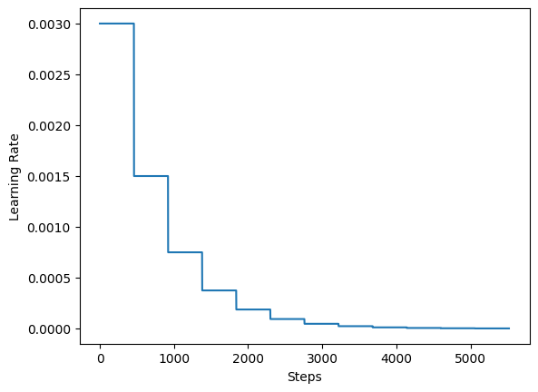
訓練
對於訓練,作者建議使用學習率排程,每 20 個 epoch 將初始學習率減半。在此範例中,我們使用 5 個 epoch。
steps_per_epoch = total_training_examples // BATCH_SIZE
total_training_steps = steps_per_epoch * EPOCHS
print(f"Steps per epoch: {steps_per_epoch}.")
print(f"Total training steps: {total_training_steps}.")

lr_schedule = keras.optimizers.schedules.ExponentialDecay(
    initial_learning_rate=0.003,
    decay_steps=steps_per_epoch * 5,
    decay_rate=0.5,
    staircase=True,
)

steps = range(total_training_steps)
lrs = [lr_schedule(step) for step in steps]

plt.plot(lrs)
plt.xlabel("Steps")
plt.ylabel("Learning Rate")
plt.show()
Steps per epoch: 92.
Total training steps: 5520.
最後,我們實作一個用於執行實驗並啟動模型訓練的實用程式。
def run_experiment(epochs):
    segmentation_model = get_shape_segmentation_model(num_points, num_classes)
    segmentation_model.compile(
        optimizer=keras.optimizers.Adam(learning_rate=lr_schedule),
        loss=keras.losses.CategoricalCrossentropy(),
        metrics=["accuracy"],
    )

    checkpoint_filepath = "checkpoint.weights.h5"
    checkpoint_callback = keras.callbacks.ModelCheckpoint(
        checkpoint_filepath,
        monitor="val_loss",
        save_best_only=True,
        save_weights_only=True,
    )

    history = segmentation_model.fit(
        train_dataset,
        validation_data=val_dataset,
        epochs=epochs,
        callbacks=[checkpoint_callback],
    )

    segmentation_model.load_weights(checkpoint_filepath)
    return segmentation_model, history


segmentation_model, history = run_experiment(epochs=EPOCHS)
Epoch 1/60
2/93 [37m━━━━━━━━━━━━━━━━━━━━ 7s 86ms/step - accuracy: 0.1427 - loss: 48748.8203
WARNING: All log messages before absl::InitializeLog() is called are written to STDERR
I0000 00:00:1699916678.434176 90326 device_compiler.h:187] Compiled cluster using XLA! This line is logged at most once for the lifetime of the process.
93/93 ━━━━━━━━━━━━━━━━━━━━ 53s 259ms/step - accuracy: 0.3739 - loss: 27980.7305 - val_accuracy: 0.4340 - val_loss: 10361231.0000
Epoch 2/60
93/93 ━━━━━━━━━━━━━━━━━━━━ 48s 82ms/step - accuracy: 0.6355 - loss: 339.9151 - val_accuracy: 0.3820 - val_loss: 19069320.0000
Epoch 3/60
93/93 ━━━━━━━━━━━━━━━━━━━━ 8s 82ms/step - accuracy: 0.6695 - loss: 281.5728 - val_accuracy: 0.2859 - val_loss: 15993839.0000
Epoch 4/60
93/93 ━━━━━━━━━━━━━━━━━━━━ 8s 89ms/step - accuracy: 0.6812 - loss: 253.0939 - val_accuracy: 0.2287 - val_loss: 9633191.0000
Epoch 5/60
93/93 ━━━━━━━━━━━━━━━━━━━━ 8s 89ms/step - accuracy: 0.6873 - loss: 231.1317 - val_accuracy: 0.3030 - val_loss: 6001454.0000
Epoch 6/60
93/93 ━━━━━━━━━━━━━━━━━━━━ 8s 88ms/step - accuracy: 0.6860 - loss: 216.6793 - val_accuracy: 0.0620 - val_loss: 1945100.8750
Epoch 7/60
93/93 ━━━━━━━━━━━━━━━━━━━━ 8s 82ms/step - accuracy: 0.6947 - loss: 210.2683 - val_accuracy: 0.4539 - val_loss: 7908162.5000
Epoch 8/60
93/93 ━━━━━━━━━━━━━━━━━━━━ 8s 82ms/step - accuracy: 0.7014 - loss: 203.2560 - val_accuracy: 0.4035 - val_loss: 17741164.0000
Epoch 9/60
93/93 ━━━━━━━━━━━━━━━━━━━━ 8s 82ms/step - accuracy: 0.7006 - loss: 197.3710 - val_accuracy: 0.1900 - val_loss: 34120616.0000
Epoch 10/60
93/93 ━━━━━━━━━━━━━━━━━━━━ 8s 82ms/step - accuracy: 0.7047 - loss: 192.0777 - val_accuracy: 0.3391 - val_loss: 33157422.0000
Epoch 11/60
93/93 ━━━━━━━━━━━━━━━━━━━━ 8s 82ms/step - accuracy: 0.7102 - loss: 188.4875 - val_accuracy: 0.3394 - val_loss: 4630613.5000
Epoch 12/60
93/93 ━━━━━━━━━━━━━━━━━━━━ 8s 89ms/step - accuracy: 0.7186 - loss: 184.9940 - val_accuracy: 0.1662 - val_loss: 487790.1250
Epoch 13/60
93/93 ━━━━━━━━━━━━━━━━━━━━ 8s 89ms/step - accuracy: 0.7175 - loss: 182.7206 - val_accuracy: 0.1602 - val_loss: 70590.3203
Epoch 14/60
93/93 ━━━━━━━━━━━━━━━━━━━━ 8s 88ms/step - accuracy: 0.7159 - loss: 180.5028 - val_accuracy: 0.1631 - val_loss: 16990.2324
Epoch 15/60
93/93 ━━━━━━━━━━━━━━━━━━━━ 8s 88ms/step - accuracy: 0.7201 - loss: 180.1674 - val_accuracy: 0.2318 - val_loss: 4992.7783
Epoch 16/60
93/93 ━━━━━━━━━━━━━━━━━━━━ 8s 88ms/step - accuracy: 0.7222 - loss: 176.5523 - val_accuracy: 0.6246 - val_loss: 647.5634
Epoch 17/60
93/93 ━━━━━━━━━━━━━━━━━━━━ 8s 88ms/step - accuracy: 0.7291 - loss: 175.6139 - val_accuracy: 0.6551 - val_loss: 324.0956
Epoch 18/60
93/93 ━━━━━━━━━━━━━━━━━━━━ 8s 88ms/step - accuracy: 0.7285 - loss: 175.0228 - val_accuracy: 0.6430 - val_loss: 257.9340
Epoch 19/60
93/93 ━━━━━━━━━━━━━━━━━━━━ 8s 88ms/step - accuracy: 0.7300 - loss: 172.7668 - val_accuracy: 0.6399 - val_loss: 253.2745
Epoch 20/60
93/93 ━━━━━━━━━━━━━━━━━━━━ 8s 89ms/step - accuracy: 0.7316 - loss: 172.9001 - val_accuracy: 0.6084 - val_loss: 232.9293
Epoch 21/60
93/93 ━━━━━━━━━━━━━━━━━━━━ 8s 89ms/step - accuracy: 0.7364 - loss: 170.8767 - val_accuracy: 0.6451 - val_loss: 191.7183
Epoch 22/60
93/93 ━━━━━━━━━━━━━━━━━━━━ 8s 88ms/step - accuracy: 0.7395 - loss: 171.4525 - val_accuracy: 0.6825 - val_loss: 180.2473
Epoch 23/60
93/93 ━━━━━━━━━━━━━━━━━━━━ 8s 82ms/step - accuracy: 0.7392 - loss: 170.1975 - val_accuracy: 0.6095 - val_loss: 180.3243
Epoch 24/60
93/93 ━━━━━━━━━━━━━━━━━━━━ 8s 88ms/step - accuracy: 0.7362 - loss: 169.2144 - val_accuracy: 0.6017 - val_loss: 178.3013
Epoch 25/60
93/93 ━━━━━━━━━━━━━━━━━━━━ 8s 82ms/step - accuracy: 0.7409 - loss: 169.2571 - val_accuracy: 0.6582 - val_loss: 178.3481
Epoch 26/60
93/93 ━━━━━━━━━━━━━━━━━━━━ 8s 89ms/step - accuracy: 0.7415 - loss: 167.7480 - val_accuracy: 0.6808 - val_loss: 177.8774
Epoch 27/60
93/93 ━━━━━━━━━━━━━━━━━━━━ 8s 89ms/step - accuracy: 0.7440 - loss: 167.7844 - val_accuracy: 0.7131 - val_loss: 176.5841
Epoch 28/60
93/93 ━━━━━━━━━━━━━━━━━━━━ 8s 88ms/step - accuracy: 0.7423 - loss: 167.5307 - val_accuracy: 0.6891 - val_loss: 176.1687
Epoch 29/60
93/93 ━━━━━━━━━━━━━━━━━━━━ 8s 88ms/step - accuracy: 0.7409 - loss: 166.4581 - val_accuracy: 0.7136 - val_loss: 174.9417
Epoch 30/60
93/93 ━━━━━━━━━━━━━━━━━━━━ 8s 88ms/step - accuracy: 0.7419 - loss: 165.9243 - val_accuracy: 0.7407 - val_loss: 173.0663
Epoch 31/60
93/93 ━━━━━━━━━━━━━━━━━━━━ 8s 88ms/step - accuracy: 0.7471 - loss: 166.9746 - val_accuracy: 0.7454 - val_loss: 172.9663
Epoch 32/60
93/93 ━━━━━━━━━━━━━━━━━━━━ 8s 82ms/step - accuracy: 0.7472 - loss: 165.9707 - val_accuracy: 0.7480 - val_loss: 173.9868
Epoch 33/60
93/93 ━━━━━━━━━━━━━━━━━━━━ 8s 82ms/step - accuracy: 0.7443 - loss: 165.9368 - val_accuracy: 0.7076 - val_loss: 174.4526
Epoch 34/60
93/93 ━━━━━━━━━━━━━━━━━━━━ 8s 82ms/step - accuracy: 0.7496 - loss: 165.5322 - val_accuracy: 0.7441 - val_loss: 174.6099
Epoch 35/60
93/93 ━━━━━━━━━━━━━━━━━━━━ 8s 82ms/step - accuracy: 0.7453 - loss: 164.2007 - val_accuracy: 0.7469 - val_loss: 174.2793
Epoch 36/60
93/93 ━━━━━━━━━━━━━━━━━━━━ 8s 82ms/step - accuracy: 0.7503 - loss: 165.3418 - val_accuracy: 0.7469 - val_loss: 174.0812
Epoch 37/60
93/93 ━━━━━━━━━━━━━━━━━━━━ 8s 82ms/step - accuracy: 0.7491 - loss: 164.4796 - val_accuracy: 0.7524 - val_loss: 173.9656
Epoch 38/60
93/93 ━━━━━━━━━━━━━━━━━━━━ 10s 82ms/step - accuracy: 0.7489 - loss: 164.4573 - val_accuracy: 0.7516 - val_loss: 175.3401
Epoch 39/60
93/93 ━━━━━━━━━━━━━━━━━━━━ 8s 82ms/step - accuracy: 0.7437 - loss: 163.4484 - val_accuracy: 0.7532 - val_loss: 173.8172
Epoch 40/60
93/93 ━━━━━━━━━━━━━━━━━━━━ 8s 82ms/step - accuracy: 0.7507 - loss: 163.6720 - val_accuracy: 0.7537 - val_loss: 173.9127
Epoch 41/60
93/93 ━━━━━━━━━━━━━━━━━━━━ 8s 82ms/step - accuracy: 0.7506 - loss: 164.0555 - val_accuracy: 0.7556 - val_loss: 173.0979
Epoch 42/60
93/93 ━━━━━━━━━━━━━━━━━━━━ 8s 89ms/step - accuracy: 0.7517 - loss: 164.1554 - val_accuracy: 0.7562 - val_loss: 172.8895
Epoch 43/60
93/93 ━━━━━━━━━━━━━━━━━━━━ 10s 82ms/step - accuracy: 0.7527 - loss: 164.6351 - val_accuracy: 0.7567 - val_loss: 173.0476
Epoch 44/60
93/93 ━━━━━━━━━━━━━━━━━━━━ 8s 88ms/step - accuracy: 0.7505 - loss: 164.1568 - val_accuracy: 0.7571 - val_loss: 172.2751
Epoch 45/60
93/93 ━━━━━━━━━━━━━━━━━━━━ 8s 88ms/step - accuracy: 0.7500 - loss: 163.8129 - val_accuracy: 0.7579 - val_loss: 171.8897
Epoch 46/60
93/93 ━━━━━━━━━━━━━━━━━━━━ 8s 82ms/step - accuracy: 0.7534 - loss: 163.6473 - val_accuracy: 0.7577 - val_loss: 172.5457
Epoch 47/60
93/93 ━━━━━━━━━━━━━━━━━━━━ 8s 82ms/step - accuracy: 0.7510 - loss: 163.7318 - val_accuracy: 0.7580 - val_loss: 172.2256
Epoch 48/60
93/93 ━━━━━━━━━━━━━━━━━━━━ 8s 82ms/step - accuracy: 0.7517 - loss: 163.3274 - val_accuracy: 0.7575 - val_loss: 172.3276
Epoch 49/60
93/93 ━━━━━━━━━━━━━━━━━━━━ 8s 89ms/step - accuracy: 0.7511 - loss: 163.5069 - val_accuracy: 0.7581 - val_loss: 171.2155
Epoch 50/60
93/93 ━━━━━━━━━━━━━━━━━━━━ 8s 89ms/step - accuracy: 0.7507 - loss: 163.7366 - val_accuracy: 0.7578 - val_loss: 171.1100
Epoch 51/60
93/93 ━━━━━━━━━━━━━━━━━━━━ 8s 82ms/step - accuracy: 0.7519 - loss: 163.1190 - val_accuracy: 0.7580 - val_loss: 171.7971
Epoch 52/60
93/93 ━━━━━━━━━━━━━━━━━━━━ 8s 81ms/step - accuracy: 0.7510 - loss: 162.7351 - val_accuracy: 0.7579 - val_loss: 171.9780
Epoch 53/60
93/93 ━━━━━━━━━━━━━━━━━━━━ 8s 82ms/step - accuracy: 0.7510 - loss: 162.9639 - val_accuracy: 0.7577 - val_loss: 171.6770
Epoch 54/60
93/93 ━━━━━━━━━━━━━━━━━━━━ 8s 88ms/step - accuracy: 0.7530 - loss: 162.7419 - val_accuracy: 0.7578 - val_loss: 170.5556
Epoch 55/60
93/93 ━━━━━━━━━━━━━━━━━━━━ 8s 82ms/step - accuracy: 0.7515 - loss: 163.2893 - val_accuracy: 0.7582 - val_loss: 171.9172
Epoch 56/60
93/93 ━━━━━━━━━━━━━━━━━━━━ 8s 82ms/step - accuracy: 0.7505 - loss: 164.2843 - val_accuracy: 0.7584 - val_loss: 171.9182
Epoch 57/60
93/93 ━━━━━━━━━━━━━━━━━━━━ 8s 82ms/step - accuracy: 0.7498 - loss: 162.6679 - val_accuracy: 0.7587 - val_loss: 173.7610
Epoch 58/60
93/93 ━━━━━━━━━━━━━━━━━━━━ 8s 82ms/step - accuracy: 0.7523 - loss: 163.3332 - val_accuracy: 0.7585 - val_loss: 172.5207
Epoch 59/60
93/93 ━━━━━━━━━━━━━━━━━━━━ 8s 82ms/step - accuracy: 0.7529 - loss: 162.4575 - val_accuracy: 0.7586 - val_loss: 171.6861
Epoch 60/60
93/93 ━━━━━━━━━━━━━━━━━━━━ 8s 82ms/step - accuracy: 0.7498 - loss: 162.9523 - val_accuracy: 0.7586 - val_loss: 172.3012
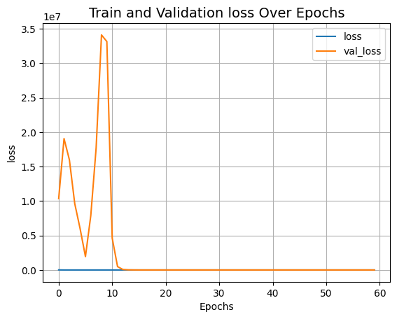
視覺化訓練情況
def plot_result(item):
plt.plot(history.history[item], label=item)
plt.plot(history.history["val_" + item], label="val_" + item)
plt.xlabel("Epochs")
plt.ylabel(item)
plt.title("Train and Validation {} Over Epochs".format(item), fontsize=14)
plt.legend()
plt.grid()
plt.show()
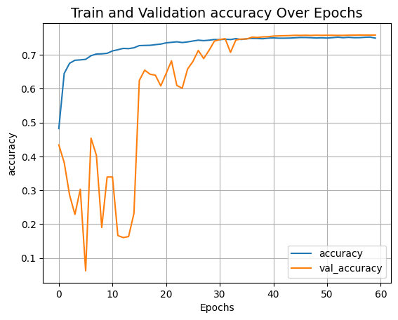
plot_result("loss")
plot_result("accuracy")
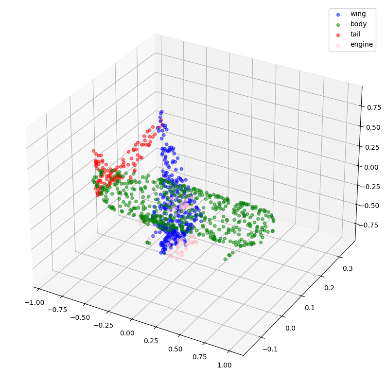
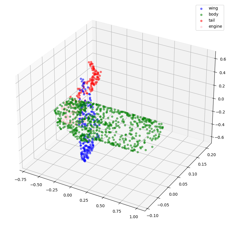
推論
validation_batch = next(iter(val_dataset))
val_predictions = segmentation_model.predict(validation_batch[0])
print(f"Validation prediction shape: {val_predictions.shape}")
def visualize_single_point_cloud(point_clouds, label_clouds, idx):
label_map = LABELS + ["none"]
point_cloud = point_clouds[idx]
label_cloud = label_clouds[idx]
visualize_data(point_cloud, [label_map[np.argmax(label)] for label in label_cloud])
idx = np.random.choice(len(validation_batch[0]))
print(f"Index selected: {idx}")
# Plotting with ground-truth.
visualize_single_point_cloud(validation_batch[0], validation_batch[1], idx)
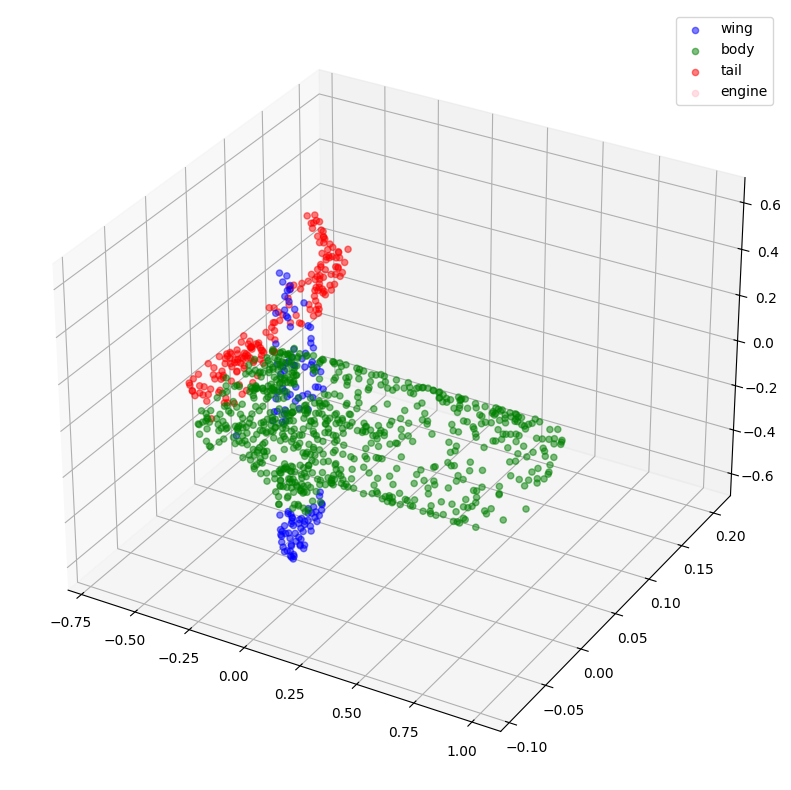
# Plotting with predicted labels.
visualize_single_point_cloud(validation_batch[0], val_predictions, idx)
 1/1 ━━━━━━━━━━━━━━━━━━━━ 1s 1s/step
Validation prediction shape: (32, 1024, 5)
Index selected: 26
最後說明
如果您有興趣了解更多關於這個主題的資訊,您可能會發現這個儲存庫很有用。