研究 Vision Transformer 的表示
作者: Aritra Roy Gosthipaty、Sayak Paul(共同貢獻)
建立日期 2022/04/12
上次修改日期 2023/11/20
描述: 研究不同的 Vision Transformer 變體所學習的表示。

簡介
在此範例中,我們將研究不同 Vision Transformer (ViT) 模型所學習的表示。本範例的主要目標是深入了解是什麼讓 ViT 能夠從圖片資料中學習。具體來說,本範例將討論幾種不同 ViT 分析工具的實作。
注意:當我們說「Vision Transformer」時,我們指的是包含 Transformer 區塊(Vaswani 等人)的電腦視覺架構,而不一定是原始的 Vision Transformer 模型(Dosovitskiy 等人)。
考量的模型
自原始 Vision Transformer 問世以來,電腦視覺社群已經出現了許多不同的 ViT 變體,以各種方式改進原始模型:訓練改進、架構改進等等。在此範例中,我們將考量以下 ViT 模型系列
- 使用 ImageNet-1k 和 ImageNet-21k 資料集進行監督預訓練的 ViT(Dosovitskiy 等人)
- 使用監督預訓練但僅使用 ImageNet-1k 資料集並具有更多正規化和蒸餾的 ViT(Touvron 等人)(DeiT)。
- 使用自我監督預訓練的 ViT(Caron 等人)(DINO)。
由於預訓練模型並未在 Keras 中實作,我們首先盡可能忠實地實作它們。然後,我們使用官方預訓練參數填充它們。最後,我們在 ImageNet-1k 驗證集上評估我們的實作,以確保評估數字與原始實作相符。我們的實作細節可在此儲存庫中找到。
為了保持範例的簡潔,我們不會詳盡地將每個模型與分析方法配對。我們會在各個章節中提供說明,以便您可以自行組合。
若要在 Google Colab 上執行此範例,我們需要更新 gdown 函式庫,如下所示
pip install -U gdown -q
匯入
import os

os.environ["KERAS_BACKEND"] = "tensorflow"

import zipfile
from io import BytesIO

import cv2
import matplotlib.pyplot as plt
import numpy as np
import requests

from PIL import Image
from sklearn.preprocessing import MinMaxScaler
import keras
from keras import ops
常數
RESOLUTION = 224
PATCH_SIZE = 16
GITHUB_RELEASE = "https://github.com/sayakpaul/probing-vits/releases/download/v1.0.0/probing_vits.zip"
FNAME = "probing_vits.zip"
MODELS_ZIP = {
    "vit_dino_base16": "Probing_ViTs/vit_dino_base16.zip",
    "vit_b16_patch16_224": "Probing_ViTs/vit_b16_patch16_224.zip",
    "vit_b16_patch16_224-i1k_pretrained": "Probing_ViTs/vit_b16_patch16_224-i1k_pretrained.zip",
}
資料公用程式
對於原始的 ViT 模型,輸入圖像需要縮放到 [-1, 1] 的範圍。對於開頭提到的其他模型系列,我們需要使用 ImageNet-1k 訓練集的通道平均值和標準差來標準化圖像。
crop_layer = keras.layers.CenterCrop(RESOLUTION, RESOLUTION)
norm_layer = keras.layers.Normalization(
    mean=[0.485 * 255, 0.456 * 255, 0.406 * 255],
    variance=[(0.229 * 255) ** 2, (0.224 * 255) ** 2, (0.225 * 255) ** 2],
)
rescale_layer = keras.layers.Rescaling(scale=1.0 / 127.5, offset=-1)


def preprocess_image(image, model_type, size=RESOLUTION):
    # Turn the image into a numpy array and add batch dim.
    image = np.array(image)
    image = ops.expand_dims(image, 0)

    # If model type is vit rescale the image to [-1, 1].
    if model_type == "original_vit":
        image = rescale_layer(image)

    # Resize the image using bicubic interpolation.
    resize_size = int((256 / 224) * size)
    image = ops.image.resize(image, (resize_size, resize_size), interpolation="bicubic")

    # Crop the image.
    image = crop_layer(image)

    # If model type is DeiT or DINO normalize the image.
    if model_type != "original_vit":
        image = norm_layer(image)

    return ops.convert_to_numpy(image)


def load_image_from_url(url, model_type):
    # Credit: Willi Gierke
    response = requests.get(url)
    image = Image.open(BytesIO(response.content))
    preprocessed_image = preprocess_image(image, model_type)
    return image, preprocessed_image
載入測試圖像並顯示它
# ImageNet-1k label mapping file and load it.
mapping_file = keras.utils.get_file(
origin="https://storage.googleapis.com/bit_models/ilsvrc2012_wordnet_lemmas.txt"
)
with open(mapping_file, "r") as f:
lines = f.readlines()
imagenet_int_to_str = [line.rstrip() for line in lines]
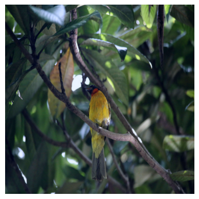
img_url = "https://dl.fbaipublicfiles.com/dino/img.png"
image, preprocessed_image = load_image_from_url(img_url, model_type="original_vit")
plt.imshow(image)
plt.axis("off")
plt.show()
載入模型
zip_path = keras.utils.get_file(
    fname=FNAME,
    origin=GITHUB_RELEASE,
)

with zipfile.ZipFile(zip_path, "r") as zip_ref:
    zip_ref.extractall("./")

os.rename("Probing ViTs", "Probing_ViTs")


def load_model(model_path: str) -> keras.Model:
    with zipfile.ZipFile(model_path, "r") as zip_ref:
        zip_ref.extractall("Probing_ViTs/")
    model_name = model_path.split(".")[0]

    inputs = keras.Input((RESOLUTION, RESOLUTION, 3))
    model = keras.layers.TFSMLayer(model_name, call_endpoint="serving_default")
    outputs = model(inputs, training=False)

    return keras.Model(inputs, outputs=outputs)


vit_base_i21k_patch16_224 = load_model(MODELS_ZIP["vit_b16_patch16_224-i1k_pretrained"])
print("Model loaded.")
Model loaded.
更多關於模型:
此模型在 ImageNet-21k 資料集上進行預訓練,然後在 ImageNet-1k 資料集上進行微調。若要瞭解更多關於我們如何在 TensorFlow 中開發此模型(使用來自 此來源的預訓練權重)的資訊,請參閱此筆記本。
使用模型執行常規推論
我們現在使用已載入的模型對我們的測試圖像執行推論。
def split_prediction_and_attention_scores(outputs):
    predictions = outputs["output_1"]
    attention_score_dict = {}
    for key, value in outputs.items():
        if key.startswith("output_2_"):
            attention_score_dict[key[len("output_2_") :]] = value
    return predictions, attention_score_dict


predictions, attention_score_dict = split_prediction_and_attention_scores(
    vit_base_i21k_patch16_224.predict(preprocessed_image)
)
predicted_label = imagenet_int_to_str[int(np.argmax(predictions))]
print(predicted_label)
 1/1 ━━━━━━━━━━━━━━━━━━━━ 5s 5s/step
toucan

WARNING: All log messages before absl::InitializeLog() is called are written to STDERR
I0000 00:00:1700526824.965785   75784 device_compiler.h:187] Compiled cluster using XLA!  This line is logged at most once for the lifetime of the process.
attention_score_dict 包含每個 Transformer 區塊中每個注意力頭的注意力分數(softmax 輸出)。
方法一:平均注意力距離
Dosovitskiy 等人和Raghu 等人使用一種稱為「平均注意力距離」的測量方法,從不同 Transformer 區塊的每個注意力頭來理解局部和全域資訊如何流入 Vision Transformer。
平均注意力距離定義為查詢權杖和其他權杖之間的距離乘以注意力權重。因此,對於單一圖像
- 我們從圖像中提取個別的圖塊(權杖),
- 計算它們的幾何距離,並
- 將其與注意力分數相乘。
注意力分數是在透過網路以推論模式傳遞圖像後計算的。下圖可能可以幫助您更好地理解此過程。

此動畫由 Ritwik Raha 製作。
def compute_distance_matrix(patch_size, num_patches, length):
    distance_matrix = np.zeros((num_patches, num_patches))
    for i in range(num_patches):
        for j in range(num_patches):
            if i == j:  # zero distance
                continue

            xi, yi = (int(i / length)), (i % length)
            xj, yj = (int(j / length)), (j % length)
            distance_matrix[i, j] = patch_size * np.linalg.norm([xi - xj, yi - yj])

    return distance_matrix


def compute_mean_attention_dist(patch_size, attention_weights, model_type):
    num_cls_tokens = 2 if "distilled" in model_type else 1

    # The attention_weights shape = (batch, num_heads, num_patches, num_patches)
    attention_weights = attention_weights[
        ..., num_cls_tokens:, num_cls_tokens:
    ]  # Removing the CLS token
    num_patches = attention_weights.shape[-1]
    length = int(np.sqrt(num_patches))
    assert length**2 == num_patches, "Num patches is not perfect square"

    distance_matrix = compute_distance_matrix(patch_size, num_patches, length)
    h, w = distance_matrix.shape

    distance_matrix = distance_matrix.reshape((1, 1, h, w))
    # The attention_weights along the last axis adds to 1
    # this is due to the fact that they are softmax of the raw logits
    # summation of the (attention_weights * distance_matrix)
    # should result in an average distance per token.
    mean_distances = attention_weights * distance_matrix
    mean_distances = np.sum(
        mean_distances, axis=-1
    )  # Sum along last axis to get average distance per token
    mean_distances = np.mean(
        mean_distances, axis=-1
    )  # Now average across all the tokens

    return mean_distances
感謝 Google 的 Simon Kornblith 協助我們提供此程式碼片段。可以在這裡找到。現在讓我們使用這些公用程式來產生一個注意力距離的圖,其中包含我們載入的模型和測試圖像。
# Build the mean distances for every Transformer block.
mean_distances = {
    f"{name}_mean_dist": compute_mean_attention_dist(
        patch_size=PATCH_SIZE,
        attention_weights=attention_weight,
        model_type="original_vit",
    )
    for name, attention_weight in attention_score_dict.items()
}

# Get the number of heads from the mean distance output.
num_heads = mean_distances["transformer_block_0_att_mean_dist"].shape[-1]

# Print the shapes
print(f"Num Heads: {num_heads}.")

plt.figure(figsize=(9, 9))

for idx in range(len(mean_distances)):
    mean_distance = mean_distances[f"transformer_block_{idx}_att_mean_dist"]
    x = [idx] * num_heads
    y = mean_distance[0, :]
    plt.scatter(x=x, y=y, label=f"transformer_block_{idx}")

plt.legend(loc="lower right")
plt.xlabel("Attention Head", fontsize=14)
plt.ylabel("Attention Distance", fontsize=14)
plt.title("vit_base_i21k_patch16_224", fontsize=14)
plt.grid()
plt.show()
Num Heads: 12.
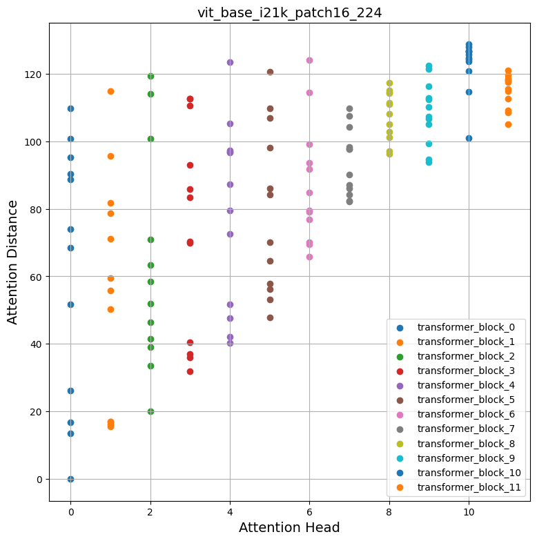
檢查圖表
自我注意力如何在輸入空間中擴展?它們是關注局部還是全域輸入區域?
自我注意力的承諾是能夠學習上下文相依性,以便模型可以關注與目標最相關的輸入區域。從上面的圖表中,我們可以注意到不同的注意力頭會產生不同的注意力距離,這表示它們會使用圖像中的局部和全域資訊。但是,當我們深入 Transformer 區塊時,這些頭傾向於更關注全域彙總資訊。
受到 Raghu 等人的啟發,我們計算了從 ImageNet-1k 驗證集中隨機選取的 1000 張圖像的平均注意力距離,並且針對開頭提到的所有模型重複了該過程。有趣的是,我們注意到以下幾點
- 使用更大的資料集進行預訓練有助於獲得更廣泛的全域注意力範圍
| 在 ImageNet-21k 上預訓練 在 ImageNet-1k 上微調 |
在 ImageNet-1k 上預訓練 |
|---|---|
- 當從 CNN 蒸餾 ViT 時,往往會減少全域注意力範圍
| 無蒸餾(DeiT 的 ViT B-16) | DeiT 的蒸餾 ViT B-16 |
|---|---|
若要重現這些圖表,請參閱此筆記本。
方法二:注意力展開
Abnar 等人引入「注意力展開」,用於量化資訊如何透過 Transformer 區塊的自我注意力層流動。原始 ViT 作者使用此方法來研究學習到的表示,聲明
簡而言之,我們將 ViTL/16 的注意力權重在所有頭上取平均值,然後遞迴地乘以所有層的權重矩陣。這說明了注意力在所有層中在權杖之間的混合。
我們使用了此筆記本,並修改了其中的注意力展開程式碼,使其與我們的模型相容。
def attention_rollout_map(image, attention_score_dict, model_type):
    num_cls_tokens = 2 if "distilled" in model_type else 1

    # Stack the individual attention matrices from individual Transformer blocks.
    attn_mat = ops.stack([attention_score_dict[k] for k in attention_score_dict.keys()])
    attn_mat = ops.squeeze(attn_mat, axis=1)

    # Average the attention weights across all heads.
    attn_mat = ops.mean(attn_mat, axis=1)

    # To account for residual connections, we add an identity matrix to the
    # attention matrix and re-normalize the weights.
    residual_attn = ops.eye(attn_mat.shape[1])
    aug_attn_mat = attn_mat + residual_attn
    aug_attn_mat = aug_attn_mat / ops.sum(aug_attn_mat, axis=-1)[..., None]
    aug_attn_mat = ops.convert_to_numpy(aug_attn_mat)

    # Recursively multiply the weight matrices.
    joint_attentions = np.zeros(aug_attn_mat.shape)
    joint_attentions[0] = aug_attn_mat[0]

    for n in range(1, aug_attn_mat.shape[0]):
        joint_attentions[n] = np.matmul(aug_attn_mat[n], joint_attentions[n - 1])

    # Attention from the output token to the input space.
    v = joint_attentions[-1]
    grid_size = int(np.sqrt(aug_attn_mat.shape[-1]))
    mask = v[0, num_cls_tokens:].reshape(grid_size, grid_size)
    mask = cv2.resize(mask / mask.max(), image.size)[..., np.newaxis]
    result = (mask * image).astype("uint8")
    return result
現在讓我們使用這些公用程式,根據我們先前從「使用模型執行常規推論」區段獲得的結果來產生注意力圖。以下是下載各個模型的連結
- 原始 ViT 模型(在 ImageNet-21k 上預訓練)
- 原始 ViT 模型(在 ImageNet-1k 上預訓練)
- DINO 模型(在 ImageNet-1k 上預訓練)
- DeiT 模型(在 ImageNet-1k 上預訓練,包括蒸餾和非蒸餾模型)
attn_rollout_result = attention_rollout_map(
    image, attention_score_dict, model_type="original_vit"
)

fig, (ax1, ax2) = plt.subplots(ncols=2, figsize=(8, 10))
fig.suptitle(f"Predicted label: {predicted_label}.", fontsize=20)

_ = ax1.imshow(image)
_ = ax2.imshow(attn_rollout_result)
ax1.set_title("Input Image", fontsize=16)
ax2.set_title("Attention Map", fontsize=16)
ax1.axis("off")
ax2.axis("off")

fig.tight_layout()
fig.subplots_adjust(top=1.35)
fig.show()
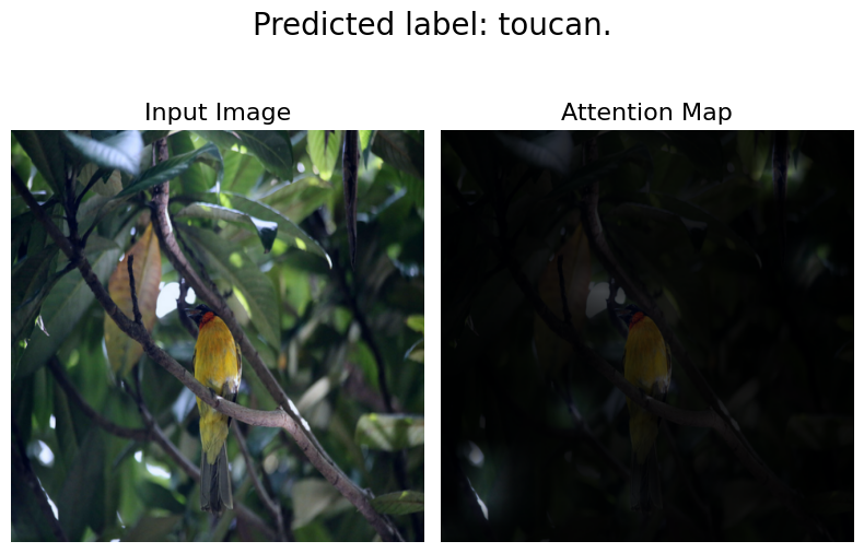
檢查圖表
我們如何量化透過注意力層傳播的資訊流?
我們注意到該模型能夠將注意力集中在輸入圖像的顯著部分。我們鼓勵您將此方法應用於我們提到的其他模型並比較結果。注意力展開圖會根據模型訓練的任務和增強而有所不同。我們觀察到 DeiT 具有最佳的展開圖,這可能是由於其增強機制所致。
方法三:注意力熱圖
一種簡單但有用的方法來探究 Vision Transformer 的表示是將注意力圖視覺化疊加在輸入圖像上。這有助於形成對模型關注內容的直覺。我們將 DINO 模型用於此目的,因為它會產生更好的注意力熱圖。
# Load the model.
vit_dino_base16 = load_model(MODELS_ZIP["vit_dino_base16"])
print("Model loaded.")

# Preprocess the same image but with normlization.
img_url = "https://dl.fbaipublicfiles.com/dino/img.png"
image, preprocessed_image = load_image_from_url(img_url, model_type="dino")

# Grab the predictions.
predictions, attention_score_dict = split_prediction_and_attention_scores(
    vit_dino_base16.predict(preprocessed_image)
)
Model loaded.
 1/1 ━━━━━━━━━━━━━━━━━━━━ 4s 4s/step
Transformer 區塊由多個頭組成。Transformer 區塊中的每個頭都會將輸入資料投射到不同的子空間。這有助於每個個別頭關注圖像的不同部分。因此,將每個注意力頭的圖分開視覺化,以了解每個頭關注的內容是有道理的。
附註:
- 以下程式碼已從原始 DINO 程式碼庫複製修改而來。
- 在這裡,我們抓取最後一個 Transformer 區塊的注意力圖。
- DINO 是使用自我監督目標進行預訓練的。
def attention_heatmap(attention_score_dict, image, model_type="dino"):
    num_tokens = 2 if "distilled" in model_type else 1

    # Sort the Transformer blocks in order of their depth.
    attention_score_list = list(attention_score_dict.keys())
    attention_score_list.sort(key=lambda x: int(x.split("_")[-2]), reverse=True)

    # Process the attention maps for overlay.
    w_featmap = image.shape[2] // PATCH_SIZE
    h_featmap = image.shape[1] // PATCH_SIZE
    attention_scores = attention_score_dict[attention_score_list[0]]

    # Taking the representations from CLS token.
    attentions = attention_scores[0, :, 0, num_tokens:].reshape(num_heads, -1)

    # Reshape the attention scores to resemble mini patches.
    attentions = attentions.reshape(num_heads, w_featmap, h_featmap)
    attentions = attentions.transpose((1, 2, 0))

    # Resize the attention patches to 224x224 (224: 14x16).
    attentions = ops.image.resize(
        attentions, size=(h_featmap * PATCH_SIZE, w_featmap * PATCH_SIZE)
    )
    return attentions
我們可以將用於 DINO 推論的同一圖像與我們從結果中提取的 attention_score_dict 一起使用。
# De-normalize the image for visual clarity.
in1k_mean = np.array([0.485 * 255, 0.456 * 255, 0.406 * 255])
in1k_std = np.array([0.229 * 255, 0.224 * 255, 0.225 * 255])
preprocessed_img_orig = (preprocessed_image * in1k_std) + in1k_mean
preprocessed_img_orig = preprocessed_img_orig / 255.0
preprocessed_img_orig = ops.convert_to_numpy(ops.clip(preprocessed_img_orig, 0.0, 1.0))

# Generate the attention heatmaps.
attentions = attention_heatmap(attention_score_dict, preprocessed_img_orig)

# Plot the maps.
fig, axes = plt.subplots(nrows=3, ncols=4, figsize=(13, 13))
img_count = 0

for i in range(3):
    for j in range(4):
        if img_count < len(attentions):
            axes[i, j].imshow(preprocessed_img_orig[0])
            axes[i, j].imshow(attentions[..., img_count], cmap="inferno", alpha=0.6)
            axes[i, j].title.set_text(f"Attention head: {img_count}")
            axes[i, j].axis("off")
            img_count += 1
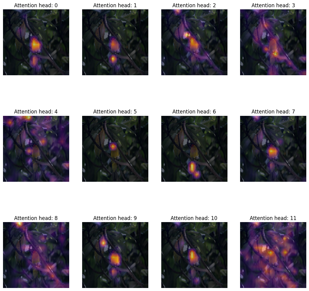
檢查圖表
我們如何定性地評估注意力權重?
Transformer 區塊的注意力權重是在鍵和查詢之間計算的。權重量化了鍵對於查詢的重要性。在 ViT 中,鍵和查詢來自同一圖像,因此權重決定了圖像的哪個部分很重要。
將疊加在圖像上的注意力權重繪製成圖,讓我們對圖像中對 Transformer 很重要的部分有了很好的直覺。此圖定性地評估了注意力權重的目的。
方法四:視覺化學習到的投射篩選器
在提取非重疊圖塊後,ViT 會在其空間維度上扁平化這些圖塊,然後線性投射它們。有人可能會想知道,這些投射看起來像什麼?在下面,我們採用 ViT B-16 模型並視覺化其學習到的投射。
def extract_weights(model, name):
    for variable in model.weights:
        if variable.name.startswith(name):
            return variable.numpy()


# Extract the projections.
projections = extract_weights(vit_base_i21k_patch16_224, "conv_projection/kernel")
projection_dim = projections.shape[-1]
patch_h, patch_w, patch_channels = projections.shape[:-1]

# Scale the projections.
scaled_projections = MinMaxScaler().fit_transform(
    projections.reshape(-1, projection_dim)
)

# Reshape the scaled projections so that the leading
# three dimensions resemble an image.
scaled_projections = scaled_projections.reshape(patch_h, patch_w, patch_channels, -1)

# Visualize the first 128 filters of the learned
# projections.
fig, axes = plt.subplots(nrows=8, ncols=16, figsize=(13, 8))
img_count = 0
limit = 128

for i in range(8):
    for j in range(16):
        if img_count < limit:
            axes[i, j].imshow(scaled_projections[..., img_count])
            axes[i, j].axis("off")
            img_count += 1

fig.tight_layout()
WARNING:matplotlib.image:Clipping input data to the valid range for imshow with RGB data ([0..1] for floats or [0..255] for integers).
WARNING:matplotlib.image:Clipping input data to the valid range for imshow with RGB data ([0..1] for floats or [0..255] for integers).
WARNING:matplotlib.image:Clipping input data to the valid range for imshow with RGB data ([0..1] for floats or [0..255] for integers).
WARNING:matplotlib.image:Clipping input data to the valid range for imshow with RGB data ([0..1] for floats or [0..255] for integers).
WARNING:matplotlib.image:Clipping input data to the valid range for imshow with RGB data ([0..1] for floats or [0..255] for integers).
WARNING:matplotlib.image:Clipping input data to the valid range for imshow with RGB data ([0..1] for floats or [0..255] for integers).
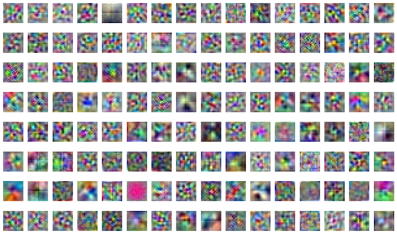
檢查圖表
投射篩選器學習了什麼?
視覺化時,卷積神經網路的核心會顯示它們在圖像中尋找的模式。這可以是圓形,有時是線條 – 當組合在一起時(在卷積網路的後期階段),篩選器會轉換成更複雜的形狀。我們發現此類卷積網路核心與 ViT 的投射篩選器之間存在驚人的相似性。
方法五:視覺化位置嵌入
Transformer 是排列不變的。這表示不考慮輸入權杖的空間位置。為了克服此限制,我們將位置資訊新增至輸入權杖。
位置資訊可以是學習的位置嵌入或手工製作的常數嵌入的形式。在我們的案例中,所有三種 ViT 變體都具有學習的位置嵌入。
在本節中,我們視覺化學習到的位置嵌入與其自身之間的相似性。在下面,我們採用 ViT B-16 模型並透過取其點積來視覺化位置嵌入的相似性。
position_embeddings = extract_weights(vit_base_i21k_patch16_224, "pos_embedding")

# Discard the batch dimension and the position embeddings of the
# cls token.
position_embeddings = position_embeddings.squeeze()[1:, ...]

similarity = position_embeddings @ position_embeddings.T
plt.imshow(similarity, cmap="inferno")
plt.show()
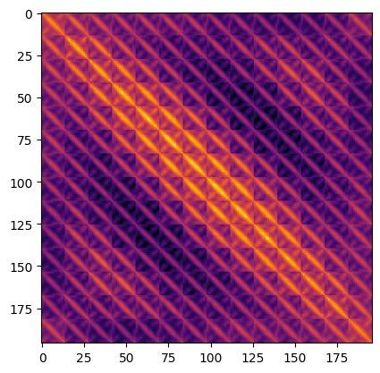
檢查圖表
位置嵌入告訴我們什麼?
該圖具有獨特的對角線圖案。主對角線最亮,表示某個位置與自身最相似。一個有趣值得關注的圖案是重複的對角線。重複的圖案描繪了一個正弦函數,該函數的本質與 Vaswani 等人提出的作為手工製作的特徵的函數非常接近。
附註
-
DINO 將注意力熱圖產生過程擴展到影片。我們也將我們的 DINO 實作應用到一系列影片中,並獲得類似的結果。這是其中一個注意力熱圖影片

- Raghu 等人使用一系列技術來研究 ViT 學習到的表示,並將其與 ResNet 的表示進行比較。我們強烈建議您閱讀他們的作品。
- 為了撰寫此範例,我們開發了此存放庫來引導我們的讀者,以便他們可以輕鬆重現實驗並擴展它們。
- 您可能會發現另一個有趣的存放庫是
vit-explain。
- 也可以使用我們的 Hugging Face 空間以自訂影像繪製注意力展開和注意力熱圖。
| 注意力熱圖 | 注意力展開 |
|---|---|