使用 SimSiam 進行自我監督對比學習
作者: Sayak Paul
建立日期 2021/03/19
上次修改日期 2023/12/29
描述: 用於電腦視覺的自我監督學習方法的實作。

自我監督學習 (SSL) 是表示學習領域中一個有趣的研究分支。SSL 系統嘗試從未標記的資料點語料庫中制定監督訊號。一個範例是我們訓練一個深度神經網路,從給定的一組詞中預測下一個詞。在文獻中,這些任務被稱為前置任務或輔助任務。如果我們在一個龐大的資料集(例如 維基百科文字語料庫)上訓練這樣的網路,它會學習非常有效的表示,這些表示可以很好地轉移到下游任務。諸如 BERT、GPT-3、ELMo 等語言模型都受益於此。
與語言模型非常相似,我們可以使用類似的方法訓練電腦視覺模型。為了在電腦視覺中實現,我們需要制定學習任務,以便底層模型(深度神經網路)能夠理解視覺資料中存在的語義資訊。其中一個任務是讓模型在同一圖像的兩個不同版本之間進行對比。希望透過這種方式,模型將學習表示,其中相似的圖像盡可能分組在一起,而不相似的圖像則更遠離。
在本範例中,我們將實作一個稱為 SimSiam 的系統,該系統在 探索簡單的連體表示學習 中提出。它的實作方式如下
- 我們使用隨機資料擴增管道建立同一資料集的兩個不同版本。請注意,在建立這些版本期間,隨機初始化種子需要相同。
- 我們取一個沒有任何分類頭部的 ResNet(主幹網路),並在其頂部添加一個淺層全連接網路(投影頭部)。總體而言,這稱為編碼器。
- 我們將編碼器的輸出傳遞到預測器,這也是一個具有類似 自動編碼器 結構的淺層全連接網路。
- 然後,我們訓練我們的編碼器,以最大化資料集兩個不同版本之間的餘弦相似度。
設定
import os
os.environ["KERAS_BACKEND"] = "tensorflow"
import keras
import keras_cv
from keras import ops

import matplotlib.pyplot as plt
import numpy as np
定義超參數
AUTO = tf.data.AUTOTUNE
BATCH_SIZE = 128
EPOCHS = 5
CROP_TO = 32
SEED = 26

PROJECT_DIM = 2048
LATENT_DIM = 512
WEIGHT_DECAY = 0.0005
載入 CIFAR-10 資料集
(x_train, y_train), (x_test, y_test) = keras.datasets.cifar10.load_data()
print(f"Total training examples: {len(x_train)}")
print(f"Total test examples: {len(x_test)}")
Total training examples: 50000
Total test examples: 10000
定義我們的資料擴增管道
如同在 SimCLR 研究中所示,擁有正確的資料增強流程對於 SSL 系統在電腦視覺中有效運作至關重要。其中兩個特別重要的增強轉換是:1.) 隨機調整大小的裁切和 2.) 色彩失真。大多數其他電腦視覺的 SSL 系統(例如 BYOL、MoCoV2、SwAV 等)都在它們的訓練流程中包含這些轉換。
strength = [0.4, 0.4, 0.4, 0.1]

random_flip = layers.RandomFlip(mode="horizontal_and_vertical")
random_crop = layers.RandomCrop(CROP_TO, CROP_TO)
random_brightness = layers.RandomBrightness(0.8 * strength[0])
random_contrast = layers.RandomContrast((1 - 0.8 * strength[1], 1 + 0.8 * strength[1]))
random_saturation = keras_cv.layers.RandomSaturation(
    (0.5 - 0.8 * strength[2], 0.5 + 0.8 * strength[2])
)
random_hue = keras_cv.layers.RandomHue(0.2 * strength[3], [0,255])
grayscale = keras_cv.layers.Grayscale()

def flip_random_crop(image):
    # With random crops we also apply horizontal flipping.
    image = random_flip(image)
    image = random_crop(image)
    return image


def color_jitter(x, strength=[0.4, 0.4, 0.3, 0.1]):
    x = random_brightness(x)
    x = random_contrast(x)
    x = random_saturation(x)
    x = random_hue(x)
    # Affine transformations can disturb the natural range of
    # RGB images, hence this is needed.
    x = ops.clip(x, 0, 255)
    return x


def color_drop(x):
    x = grayscale(x)
    x = ops.tile(x, [1, 1, 3])
    return x


def random_apply(func, x, p):
    if keras.random.uniform([], minval=0, maxval=1) < p:
        return func(x)
    else:
        return x


def custom_augment(image):
    # As discussed in the SimCLR paper, the series of augmentation
    # transformations (except for random crops) need to be applied
    # randomly to impose translational invariance.
    image = flip_random_crop(image)
    image = random_apply(color_jitter, image, p=0.8)
    image = random_apply(color_drop, image, p=0.2)
    return image
應該注意的是,資料增強流程通常取決於我們正在處理的資料集的各種屬性。例如,如果資料集中的影像以物件為中心,那麼以非常高的機率進行隨機裁切可能會損害訓練效能。
現在讓我們將資料增強流程應用於我們的資料集,並視覺化一些輸出結果。
將資料轉換為 TensorFlow Dataset 物件
在這裡,我們建立兩個不同版本的資料集,沒有任何真實標籤。
ssl_ds_one = tf.data.Dataset.from_tensor_slices(x_train)
ssl_ds_one = (
    ssl_ds_one.shuffle(1024, seed=SEED)
    .map(custom_augment, num_parallel_calls=AUTO)
    .batch(BATCH_SIZE)
    .prefetch(AUTO)
)

ssl_ds_two = tf.data.Dataset.from_tensor_slices(x_train)
ssl_ds_two = (
    ssl_ds_two.shuffle(1024, seed=SEED)
    .map(custom_augment, num_parallel_calls=AUTO)
    .batch(BATCH_SIZE)
    .prefetch(AUTO)
)

# We then zip both of these datasets.
ssl_ds = tf.data.Dataset.zip((ssl_ds_one, ssl_ds_two))

# Visualize a few augmented images.
sample_images_one = next(iter(ssl_ds_one))
plt.figure(figsize=(10, 10))
for n in range(25):
    ax = plt.subplot(5, 5, n + 1)
    plt.imshow(sample_images_one[n].numpy().astype("int"))
    plt.axis("off")
plt.show()

# Ensure that the different versions of the dataset actually contain
# identical images.
sample_images_two = next(iter(ssl_ds_two))
plt.figure(figsize=(10, 10))
for n in range(25):
    ax = plt.subplot(5, 5, n + 1)
    plt.imshow(sample_images_two[n].numpy().astype("int"))
    plt.axis("off")
plt.show()
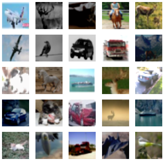
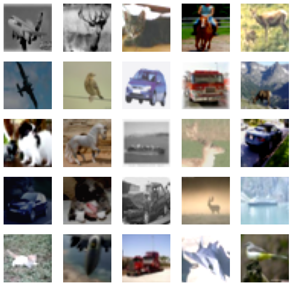
請注意,samples_images_one 和 sample_images_two 中的影像本質上相同,但增強方式不同。
定義編碼器和預測器
我們使用專為 CIFAR10 資料集配置的 ResNet20 實作。程式碼取自 keras-idiomatic-programmer 儲存庫。這些架構的超參數參考自 原始論文 的第 3 節和附錄 A。
!wget -q https://git.io/JYx2x -O resnet_cifar10_v2.py
import resnet_cifar10_v2

N = 2
DEPTH = N * 9 + 2
NUM_BLOCKS = ((DEPTH - 2) // 9) - 1


def get_encoder():
    # Input and backbone.
    inputs = layers.Input((CROP_TO, CROP_TO, 3))
    x = layers.Rescaling(scale=1.0 / 127.5, offset=-1)(
        inputs
    )
    x = resnet_cifar10_v2.stem(x)
    x = resnet_cifar10_v2.learner(x, NUM_BLOCKS)
    x = layers.GlobalAveragePooling2D(name="backbone_pool")(x)

    # Projection head.
    x = layers.Dense(
        PROJECT_DIM, use_bias=False, kernel_regularizer=regularizers.l2(WEIGHT_DECAY)
    )(x)
    x = layers.BatchNormalization()(x)
    x = layers.ReLU()(x)
    x = layers.Dense(
        PROJECT_DIM, use_bias=False, kernel_regularizer=regularizers.l2(WEIGHT_DECAY)
    )(x)
    outputs = layers.BatchNormalization()(x)
    return keras.Model(inputs, outputs, name="encoder")


def get_predictor():
    model = keras.Sequential(
        [
            # Note the AutoEncoder-like structure.
            layers.Input((PROJECT_DIM,)),
            layers.Dense(
                LATENT_DIM,
                use_bias=False,
                kernel_regularizer=regularizers.l2(WEIGHT_DECAY),
            ),
            layers.ReLU(),
            layers.BatchNormalization(),
            layers.Dense(PROJECT_DIM),
        ],
        name="predictor",
    )
    return model
定義(預)訓練迴圈
使用這些方法訓練網路的主要原因之一是利用學習到的表示來執行下游任務,例如分類。這也是為什麼這個特定的訓練階段也被稱為預訓練的原因。
我們先定義損失函數。
def compute_loss(p, z):
    # The authors of SimSiam emphasize the impact of
    # the `stop_gradient` operator in the paper as it
    # has an important role in the overall optimization.
    z = ops.stop_gradient(z)
    p = keras.utils.normalize(p, axis=1, order=2)
    z = keras.utils.normalize(z, axis=1, order=2)
    # Negative cosine similarity (minimizing this is
    # equivalent to maximizing the similarity).
    return -ops.mean(ops.sum((p * z), axis=1))
然後,我們透過覆寫 keras.Model 類別的 train_step() 函數來定義我們的訓練迴圈。
class SimSiam(keras.Model):
    def __init__(self, encoder, predictor):
        super().__init__()
        self.encoder = encoder
        self.predictor = predictor
        self.loss_tracker = keras.metrics.Mean(name="loss")

    @property
    def metrics(self):
        return [self.loss_tracker]

    def train_step(self, data):
        # Unpack the data.
        ds_one, ds_two = data

        # Forward pass through the encoder and predictor.
        with tf.GradientTape() as tape:
            z1, z2 = self.encoder(ds_one), self.encoder(ds_two)
            p1, p2 = self.predictor(z1), self.predictor(z2)
            # Note that here we are enforcing the network to match
            # the representations of two differently augmented batches
            # of data.
            loss = compute_loss(p1, z2) / 2 + compute_loss(p2, z1) / 2

        # Compute gradients and update the parameters.
        learnable_params = (
            self.encoder.trainable_variables + self.predictor.trainable_variables
        )
        gradients = tape.gradient(loss, learnable_params)
        self.optimizer.apply_gradients(zip(gradients, learnable_params))

        # Monitor loss.
        self.loss_tracker.update_state(loss)
        return {"loss": self.loss_tracker.result()}
預訓練我們的網路
為了這個範例的緣故,我們只會訓練模型 5 個 epoch。實際上,這至少應該是 100 個 epoch。
# Create a cosine decay learning scheduler.
num_training_samples = len(x_train)
steps = EPOCHS * (num_training_samples // BATCH_SIZE)
lr_decayed_fn = keras.optimizers.schedules.CosineDecay(
    initial_learning_rate=0.03, decay_steps=steps
)

# Create an early stopping callback.
early_stopping = keras.callbacks.EarlyStopping(
    monitor="loss", patience=5, restore_best_weights=True
)

# Compile model and start training.
simsiam = SimSiam(get_encoder(), get_predictor())
simsiam.compile(optimizer=keras.optimizers.SGD(lr_decayed_fn, momentum=0.6))
history = simsiam.fit(ssl_ds, epochs=EPOCHS, callbacks=[early_stopping])

# Visualize the training progress of the model.
plt.plot(history.history["loss"])
plt.grid()
plt.title("Negative Cosine Similairty")
plt.show()
Epoch 1/5
391/391 [==============================] - 33s 42ms/step - loss: -0.8973
Epoch 2/5
391/391 [==============================] - 16s 40ms/step - loss: -0.9129
Epoch 3/5
391/391 [==============================] - 16s 40ms/step - loss: -0.9165
Epoch 4/5
391/391 [==============================] - 16s 40ms/step - loss: -0.9176
Epoch 5/5
391/391 [==============================] - 16s 40ms/step - loss: -0.9182
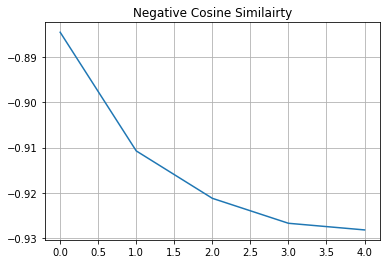
如果您的解決方案在不同的資料集和不同的主幹架構下,很快就非常接近 -1(我們損失的最小值),那很可能是因為表示崩潰。這是一種編碼器為所有影像產生類似輸出的現象。在這種情況下,需要額外的超參數調整,尤其是在以下方面:
- 色彩失真的強度及其機率。
- 學習率及其排程。
- 主幹及其投影頭的架構。
評估我們的 SSL 方法
在電腦視覺中評估 SSL 方法(或任何其他預訓練方法)最常用的方法是在已訓練的主幹模型(在本例中為 ResNet20)的凍結特徵上學習一個線性分類器,並在未見過的影像上評估該分類器。其他方法包括在原始資料集上或甚至在有 5% 或 10% 標籤的目標資料集上進行 微調。實際上,我們可以將主幹模型用於任何下游任務,例如語義分割、物件偵測等等,其中主幹模型通常使用純監督學習進行預訓練。
# We first create labeled `Dataset` objects.
train_ds = tf.data.Dataset.from_tensor_slices((x_train, y_train))
test_ds = tf.data.Dataset.from_tensor_slices((x_test, y_test))

# Then we shuffle, batch, and prefetch this dataset for performance. We
# also apply random resized crops as an augmentation but only to the
# training set.
train_ds = (
    train_ds.shuffle(1024)
    .map(lambda x, y: (flip_random_crop(x), y), num_parallel_calls=AUTO)
    .batch(BATCH_SIZE)
    .prefetch(AUTO)
)
test_ds = test_ds.batch(BATCH_SIZE).prefetch(AUTO)

# Extract the backbone ResNet20.
backbone = keras.Model(
    simsiam.encoder.input, simsiam.encoder.get_layer("backbone_pool").output
)

# We then create our linear classifier and train it.
backbone.trainable = False
inputs = layers.Input((CROP_TO, CROP_TO, 3))
x = backbone(inputs, training=False)
outputs = layers.Dense(10, activation="softmax")(x)
linear_model = keras.Model(inputs, outputs, name="linear_model")

# Compile model and start training.
linear_model.compile(
    loss="sparse_categorical_crossentropy",
    metrics=["accuracy"],
    optimizer=keras.optimizers.SGD(lr_decayed_fn, momentum=0.9),
)
history = linear_model.fit(
    train_ds, validation_data=test_ds, epochs=EPOCHS, callbacks=[early_stopping]
)
_, test_acc = linear_model.evaluate(test_ds)
print("Test accuracy: {:.2f}%".format(test_acc * 100))
Epoch 1/5
391/391 [==============================] - 7s 11ms/step - loss: 3.8072 - accuracy: 0.1527 - val_loss: 3.7449 - val_accuracy: 0.2046
Epoch 2/5
391/391 [==============================] - 3s 8ms/step - loss: 3.7356 - accuracy: 0.2107 - val_loss: 3.7055 - val_accuracy: 0.2308
Epoch 3/5
391/391 [==============================] - 3s 8ms/step - loss: 3.7036 - accuracy: 0.2228 - val_loss: 3.6874 - val_accuracy: 0.2329
Epoch 4/5
391/391 [==============================] - 3s 8ms/step - loss: 3.6893 - accuracy: 0.2276 - val_loss: 3.6808 - val_accuracy: 0.2334
Epoch 5/5
391/391 [==============================] - 3s 9ms/step - loss: 3.6845 - accuracy: 0.2305 - val_loss: 3.6798 - val_accuracy: 0.2339
79/79 [==============================] - 1s 7ms/step - loss: 3.6798 - accuracy: 0.2339
Test accuracy: 23.39%