視覺化卷積網路的學習內容
作者: fchollet
建立日期 2020/05/29
最後修改日期 2020/05/29
描述: 顯示卷積網路濾波器響應的視覺模式。

簡介
在此範例中,我們將探討圖像分類模型學習的視覺模式類型。我們將使用在 ImageNet 數據集上訓練的 ResNet50V2 模型。
我們的流程很簡單:我們將建立輸入圖像,以最大化目標層中特定濾波器的活化 (選取模型中間的某個位置:層 conv3_block4_out)。此類圖像表示濾波器響應的模式視覺化。
設定
import os

os.environ["KERAS_BACKEND"] = "tensorflow"

import keras
import numpy as np
import tensorflow as tf

# The dimensions of our input image
img_width = 180
img_height = 180
# Our target layer: we will visualize the filters from this layer.
# See `model.summary()` for list of layer names, if you want to change this.
layer_name = "conv3_block4_out"
建立特徵提取模型
# Build a ResNet50V2 model loaded with pre-trained ImageNet weights
model = keras.applications.ResNet50V2(weights="imagenet", include_top=False)

# Set up a model that returns the activation values for our target layer
layer = model.get_layer(name=layer_name)
feature_extractor = keras.Model(inputs=model.inputs, outputs=layer.output)
設定梯度上升流程
我們將最大化的「損失」僅為目標層中特定濾波器活化的平均值。為避免邊界效應,我們排除邊界像素。
def compute_loss(input_image, filter_index):
    activation = feature_extractor(input_image)
    # We avoid border artifacts by only involving non-border pixels in the loss.
    filter_activation = activation[:, 2:-2, 2:-2, filter_index]
    return tf.reduce_mean(filter_activation)
我們的梯度上升函數只計算以上損失相對於輸入圖像的梯度,並更新更新圖像,使其朝向更強烈活化目標濾波器的狀態移動。
@tf.function
def gradient_ascent_step(img, filter_index, learning_rate):
    with tf.GradientTape() as tape:
        tape.watch(img)
        loss = compute_loss(img, filter_index)
    # Compute gradients.
    grads = tape.gradient(loss, img)
    # Normalize gradients.
    grads = tf.math.l2_normalize(grads)
    img += learning_rate * grads
    return loss, img
設定端對端濾波器視覺化迴圈
我們的流程如下
- 從接近「全灰」 (即視覺上中性) 的隨機圖像開始
- 重複套用以上定義的梯度上升步驟函數
- 透過正規化、中心裁剪並將其限制在 [0, 255] 範圍內,將產生的輸入圖像轉換回可顯示的形式。
def initialize_image():
    # We start from a gray image with some random noise
    img = tf.random.uniform((1, img_width, img_height, 3))
    # ResNet50V2 expects inputs in the range [-1, +1].
    # Here we scale our random inputs to [-0.125, +0.125]
    return (img - 0.5) * 0.25


def visualize_filter(filter_index):
    # We run gradient ascent for 20 steps
    iterations = 30
    learning_rate = 10.0
    img = initialize_image()
    for iteration in range(iterations):
        loss, img = gradient_ascent_step(img, filter_index, learning_rate)

    # Decode the resulting input image
    img = deprocess_image(img[0].numpy())
    return loss, img


def deprocess_image(img):
    # Normalize array: center on 0., ensure variance is 0.15
    img -= img.mean()
    img /= img.std() + 1e-5
    img *= 0.15

    # Center crop
    img = img[25:-25, 25:-25, :]

    # Clip to [0, 1]
    img += 0.5
    img = np.clip(img, 0, 1)

    # Convert to RGB array
    img *= 255
    img = np.clip(img, 0, 255).astype("uint8")
    return img
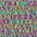
讓我們試試目標層中的濾波器 0
from IPython.display import Image, display

loss, img = visualize_filter(0)
keras.utils.save_img("0.png", img)
這是最大化目標層中濾波器 0 響應的輸入外觀
display(Image("0.png"))
視覺化目標層中的前 64 個濾波器
現在,讓我們製作目標層中前 64 個濾波器的 8x8 格網,以了解模型學習的不同視覺模式的範圍。
# Compute image inputs that maximize per-filter activations
# for the first 64 filters of our target layer
all_imgs = []
for filter_index in range(64):
    print("Processing filter %d" % (filter_index,))
    loss, img = visualize_filter(filter_index)
    all_imgs.append(img)

# Build a black picture with enough space for
# our 8 x 8 filters of size 128 x 128, with a 5px margin in between
margin = 5
n = 8
cropped_width = img_width - 25 * 2
cropped_height = img_height - 25 * 2
width = n * cropped_width + (n - 1) * margin
height = n * cropped_height + (n - 1) * margin
stitched_filters = np.zeros((width, height, 3))

# Fill the picture with our saved filters
for i in range(n):
    for j in range(n):
        img = all_imgs[i * n + j]
        stitched_filters[
            (cropped_width + margin) * i : (cropped_width + margin) * i + cropped_width,
            (cropped_height + margin) * j : (cropped_height + margin) * j
            + cropped_height,
            :,
        ] = img
keras.utils.save_img("stiched_filters.png", stitched_filters)

from IPython.display import Image, display

display(Image("stiched_filters.png"))
Processing filter 0
Processing filter 1
Processing filter 2
Processing filter 3
Processing filter 4
Processing filter 5
Processing filter 6
Processing filter 7
Processing filter 8
Processing filter 9
Processing filter 10
Processing filter 11
Processing filter 12
Processing filter 13
Processing filter 14
Processing filter 15
Processing filter 16
Processing filter 17
Processing filter 18
Processing filter 19
Processing filter 20
Processing filter 21
Processing filter 22
Processing filter 23
Processing filter 24
Processing filter 25
Processing filter 26
Processing filter 27
Processing filter 28
Processing filter 29
Processing filter 30
Processing filter 31
Processing filter 32
Processing filter 33
Processing filter 34
Processing filter 35
Processing filter 36
Processing filter 37
Processing filter 38
Processing filter 39
Processing filter 40
Processing filter 41
Processing filter 42
Processing filter 43
Processing filter 44
Processing filter 45
Processing filter 46
Processing filter 47
Processing filter 48
Processing filter 49
Processing filter 50
Processing filter 51
Processing filter 52
Processing filter 53
Processing filter 54
Processing filter 55
Processing filter 56
Processing filter 57
Processing filter 58
Processing filter 59
Processing filter 60
Processing filter 61
Processing filter 62
Processing filter 63
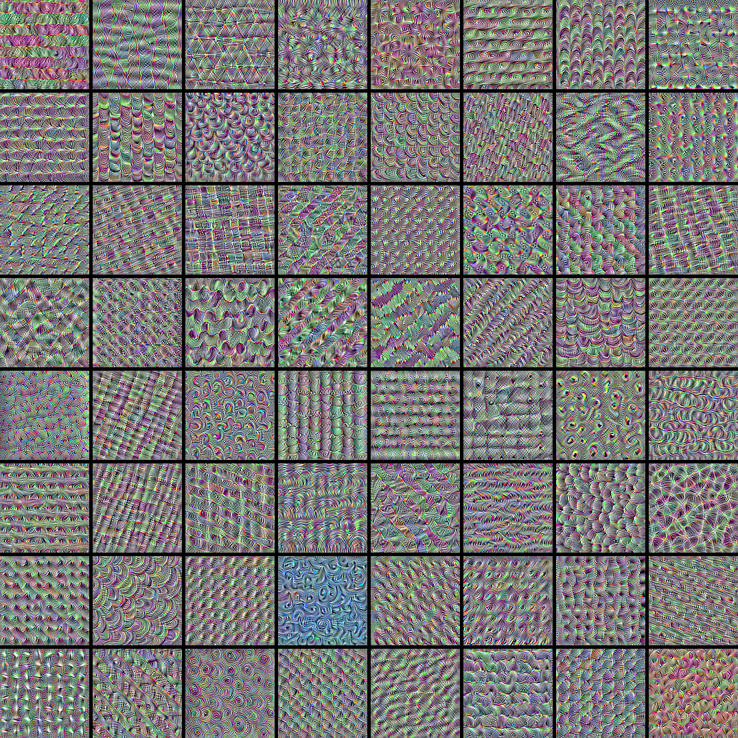
圖像分類模型會透過將其輸入分解到此類紋理濾波器的「向量基礎」上來觀察世界。
另請參閱這篇舊的部落格文章以了解分析和解釋。