使用 YOLOV8 和 KerasCV 實現高效物件偵測
作者: Gitesh Chawda
建立日期 2023/06/26
最後修改日期 2023/06/26
描述: 使用 KerasCV 訓練自訂 YOLOV8 物件偵測模型。

簡介
KerasCV 是 Keras 的擴充,用於電腦視覺任務。在本範例中,我們將了解如何使用 KerasCV 訓練 YOLOV8 物件偵測模型。
KerasCV 包含用於熱門電腦視覺資料集 (例如 ImageNet、COCO 和 Pascal VOC) 的預訓練模型,這些模型可用於遷移學習。KerasCV 也提供一系列視覺化工具,用於檢查模型學習的中間表示,以及視覺化物件偵測和分割任務的結果。
如果您有興趣了解如何使用 KerasCV 進行物件偵測,我強烈建議您查看 lukewood 建立的指南。此資源可在 使用 KerasCV 進行物件偵測 找到,其中全面概述了使用 KerasCV 建立物件偵測模型所需的基本概念和技術。
!pip install --upgrade git+https://github.com/keras-team/keras-cv -q
[33mWARNING: Running pip as the 'root' user can result in broken permissions and conflicting behaviour with the system package manager. It is recommended to use a virtual environment instead: https://pip.dev.org.tw/warnings/venv[0m[33m
[0m
設定
import os
from tqdm.auto import tqdm
import xml.etree.ElementTree as ET

import tensorflow as tf
from tensorflow import keras

import keras_cv
from keras_cv import bounding_box
from keras_cv import visualization
/opt/conda/lib/python3.10/site-packages/tensorflow_io/python/ops/__init__.py:98: UserWarning: unable to load libtensorflow_io_plugins.so: unable to open file: libtensorflow_io_plugins.so, from paths: ['/opt/conda/lib/python3.10/site-packages/tensorflow_io/python/ops/libtensorflow_io_plugins.so']
caused by: ['/opt/conda/lib/python3.10/site-packages/tensorflow_io/python/ops/libtensorflow_io_plugins.so: undefined symbol: _ZN3tsl6StatusC1EN10tensorflow5error4CodeESt17basic_string_viewIcSt11char_traitsIcEENS_14SourceLocationE']
  warnings.warn(f"unable to load libtensorflow_io_plugins.so: {e}")
/opt/conda/lib/python3.10/site-packages/tensorflow_io/python/ops/__init__.py:104: UserWarning: file system plugins are not loaded: unable to open file: libtensorflow_io.so, from paths: ['/opt/conda/lib/python3.10/site-packages/tensorflow_io/python/ops/libtensorflow_io.so']
caused by: ['/opt/conda/lib/python3.10/site-packages/tensorflow_io/python/ops/libtensorflow_io.so: undefined symbol: _ZTVN10tensorflow13GcsFileSystemE']
  warnings.warn(f"file system plugins are not loaded: {e}")
載入資料
在本指南中,我們將使用從 roboflow 取得的自駕車資料集。為了使資料集更易於管理,我已提取較大資料集的一個子集,該資料集最初包含 15,000 個資料樣本。在此子集中,我選擇了 7,316 個樣本用於模型訓練。
為了簡化手邊的任務並集中精力,我們將使用減少的物件類別數量。具體來說,我們將考慮五個主要的偵測和分類類別:汽車、行人、交通號誌、自行車騎士和卡車。這些類別代表自駕車環境中最常見和最重要的物件。
透過將資料集縮減為這些特定類別,我們可以專注於建立強大的物件偵測模型,該模型可以準確識別和分類這些重要物件。
TensorFlow Datasets 函式庫提供了一種方便的方式來下載和使用各種資料集,包括物件偵測資料集。對於那些想要快速開始使用資料而無需手動下載和預處理資料的人來說,這是一個絕佳的選擇。
您可以在這裡查看各種物件偵測資料集:TensorFlow 資料集
然而,在這個程式碼範例中,我們將示範如何使用 TensorFlow 的 tf.data 管線從頭開始載入資料集。這種方法提供了更大的彈性,並允許您根據需要自訂預處理步驟。
載入 TensorFlow Datasets 函式庫中沒有提供的自訂資料集是使用 tf.data 管線的主要優勢之一。這種方法允許您創建一個客製化的資料預處理管線,以滿足您的資料集的特定需求和要求。
超參數
SPLIT_RATIO = 0.2
BATCH_SIZE = 4
LEARNING_RATE = 0.001
EPOCH = 5
GLOBAL_CLIPNORM = 10.0
建立一個字典,將每個類別名稱對應到一個唯一的數字識別碼。這個對應在物件偵測任務的訓練和推論期間,用於編碼和解碼類別標籤。
class_ids = [
    "car",
    "pedestrian",
    "trafficLight",
    "biker",
    "truck",
]
class_mapping = dict(zip(range(len(class_ids)), class_ids))

# Path to images and annotations
path_images = "/kaggle/input/dataset/data/images/"
path_annot = "/kaggle/input/dataset/data/annotations/"

# Get all XML file paths in path_annot and sort them
xml_files = sorted(
    [
        os.path.join(path_annot, file_name)
        for file_name in os.listdir(path_annot)
        if file_name.endswith(".xml")
    ]
)

# Get all JPEG image file paths in path_images and sort them
jpg_files = sorted(
    [
        os.path.join(path_images, file_name)
        for file_name in os.listdir(path_images)
        if file_name.endswith(".jpg")
    ]
)
以下函式會讀取 XML 檔案,並找到影像名稱和路徑,然後迭代 XML 檔案中的每個物件,以提取每個物件的邊界框座標和類別標籤。
此函式會回傳三個值:影像路徑、邊界框列表(每個邊界框表示為四個浮點數的列表:xmin、ymin、xmax、ymax)以及對應每個邊界框的類別 ID 列表(表示為整數)。類別 ID 是透過使用名為 class_mapping 的字典,將類別標籤對應到整數值而取得的。
def parse_annotation(xml_file):
    tree = ET.parse(xml_file)
    root = tree.getroot()

    image_name = root.find("filename").text
    image_path = os.path.join(path_images, image_name)

    boxes = []
    classes = []
    for obj in root.iter("object"):
        cls = obj.find("name").text
        classes.append(cls)

        bbox = obj.find("bndbox")
        xmin = float(bbox.find("xmin").text)
        ymin = float(bbox.find("ymin").text)
        xmax = float(bbox.find("xmax").text)
        ymax = float(bbox.find("ymax").text)
        boxes.append([xmin, ymin, xmax, ymax])

    class_ids = [
        list(class_mapping.keys())[list(class_mapping.values()).index(cls)]
        for cls in classes
    ]
    return image_path, boxes, class_ids


image_paths = []
bbox = []
classes = []
for xml_file in tqdm(xml_files):
    image_path, boxes, class_ids = parse_annotation(xml_file)
    image_paths.append(image_path)
    bbox.append(boxes)
    classes.append(class_ids)
0%| | 0/7316 [00:00<?, ?it/s]
這裡我們使用 tf.ragged.constant 從 bbox 和 classes 列表建立不規則張量。不規則張量是一種可以處理沿著一或多個維度具有可變長度資料的張量類型。當處理具有可變長度序列的資料(例如文字或時間序列資料)時,這非常有用。
classes = [
    [8, 8, 8, 8, 8],      # 5 classes
    [12, 14, 14, 14],     # 4 classes
    [1],                  # 1 class
    [7, 7],               # 2 classes
 ...]
bbox = [
    [[199.0, 19.0, 390.0, 401.0],
    [217.0, 15.0, 270.0, 157.0],
    [393.0, 18.0, 432.0, 162.0],
    [1.0, 15.0, 226.0, 276.0],
    [19.0, 95.0, 458.0, 443.0]],     #image 1 has 4 objects
    [[52.0, 117.0, 109.0, 177.0]],   #image 2 has 1 object
    [[88.0, 87.0, 235.0, 322.0],
    [113.0, 117.0, 218.0, 471.0]],   #image 3 has 2 objects
 ...]
在這個例子中,bbox 和 classes 列表對於每個影像都有不同的長度,這取決於影像中的物件數量以及對應的邊界框和類別。為了處理這種可變性,我們使用不規則張量而不是常規張量。
稍後,這些不規則張量會使用 from_tensor_slices 方法建立 tf.data.Dataset。此方法透過沿著第一個維度切片輸入張量來從輸入張量建立資料集。透過使用不規則張量,資料集可以處理每個影像的可變長度資料,並為進一步的處理提供彈性的輸入管線。
bbox = tf.ragged.constant(bbox)
classes = tf.ragged.constant(classes)
image_paths = tf.ragged.constant(image_paths)

data = tf.data.Dataset.from_tensor_slices((image_paths, classes, bbox))
將資料分成訓練資料和驗證資料
# Determine the number of validation samples
num_val = int(len(xml_files) * SPLIT_RATIO)

# Split the dataset into train and validation sets
val_data = data.take(num_val)
train_data = data.skip(num_val)
讓我們看看資料載入和邊界框格式化的部分,讓事情順利進行。KerasCV 中的邊界框具有預定的格式。為此,您必須將邊界框綑綁到符合下列要求的字典中
bounding_boxes = {
    # num_boxes may be a Ragged dimension
    'boxes': Tensor(shape=[batch, num_boxes, 4]),
    'classes': Tensor(shape=[batch, num_boxes])
}
該字典有兩個鍵,'boxes' 和 'classes',每個鍵都對應到 TensorFlow RaggedTensor 或 Tensor 物件。 'boxes' 張量的形狀為 [batch, num_boxes, 4],其中 batch 是批次中的影像數量,而 num_boxes 是任何影像中邊界框的最大數量。 4 代表定義邊界框所需的四個值:xmin、ymin、xmax、ymax。
'classes' 張量的形狀為 [batch, num_boxes],其中每個元素都代表 'boxes' 張量中對應邊界框的類別標籤。num_boxes 維度可能是不規則的,這表示批次中影像的框數可能會有所不同。
最終的字典應該是
{"images": images, "bounding_boxes": bounding_boxes}
def load_image(image_path):
    image = tf.io.read_file(image_path)
    image = tf.image.decode_jpeg(image, channels=3)
    return image


def load_dataset(image_path, classes, bbox):
    # Read Image
    image = load_image(image_path)
    bounding_boxes = {
        "classes": tf.cast(classes, dtype=tf.float32),
        "boxes": bbox,
    }
    return {"images": tf.cast(image, tf.float32), "bounding_boxes": bounding_boxes}
這裡我們建立一個層,將影像大小調整為 640x640 像素,同時保持原始的長寬比。與影像相關聯的邊界框以 xyxy 格式指定。如有必要,將會用零填充調整大小後的影像,以保持原始的長寬比。
KerasCV 支援的邊界框格式:1. CENTER_XYWH 2. XYWH 3. XYXY 4. REL_XYXY 5. REL_XYWH 6. YXYX 7. REL_YXYX
您可以在 docs 中閱讀更多有關 KerasCV 邊界框格式的資訊。
此外,可以執行任意兩個配對之間的格式轉換
boxes = keras_cv.bounding_box.convert_format(
        bounding_box,
        images=image,
        source="xyxy",  # Original Format
        target="xywh",  # Target Format (to which we want to convert)
    )
資料擴增
建構物件偵測管線時,最具挑戰性的任務之一是資料擴增。它涉及對輸入影像應用各種轉換,以增加訓練資料的多樣性,並提高模型泛化的能力。然而,當處理物件偵測任務時,它會變得更加複雜,因為這些轉換需要知道底層的邊界框,並相應地更新它們。
KerasCV 提供對邊界框擴增的本地支援。KerasCV 提供了大量專門設計用於處理邊界框的資料擴增層。當影像轉換時,這些層會智慧地調整邊界框座標,確保邊界框保持精確,並與擴增的影像對齊。
透過利用 KerasCV 的功能,開發人員可以方便地將對邊界框友好的資料擴增整合到其物件偵測管線中。透過在 tf.data 管線內執行即時擴增,該過程變得無縫且有效率,從而實現更好的訓練和更準確的物件偵測結果。
augmenter = keras.Sequential(
    layers=[
        keras_cv.layers.RandomFlip(mode="horizontal", bounding_box_format="xyxy"),
        keras_cv.layers.RandomShear(
            x_factor=0.2, y_factor=0.2, bounding_box_format="xyxy"
        ),
        keras_cv.layers.JitteredResize(
            target_size=(640, 640), scale_factor=(0.75, 1.3), bounding_box_format="xyxy"
        ),
    ]
)
建立訓練資料集
train_ds = train_data.map(load_dataset, num_parallel_calls=tf.data.AUTOTUNE)
train_ds = train_ds.shuffle(BATCH_SIZE * 4)
train_ds = train_ds.ragged_batch(BATCH_SIZE, drop_remainder=True)
train_ds = train_ds.map(augmenter, num_parallel_calls=tf.data.AUTOTUNE)
建立驗證資料集
resizing = keras_cv.layers.JitteredResize(
    target_size=(640, 640),
    scale_factor=(0.75, 1.3),
    bounding_box_format="xyxy",
)

val_ds = val_data.map(load_dataset, num_parallel_calls=tf.data.AUTOTUNE)
val_ds = val_ds.shuffle(BATCH_SIZE * 4)
val_ds = val_ds.ragged_batch(BATCH_SIZE, drop_remainder=True)
val_ds = val_ds.map(resizing, num_parallel_calls=tf.data.AUTOTUNE)
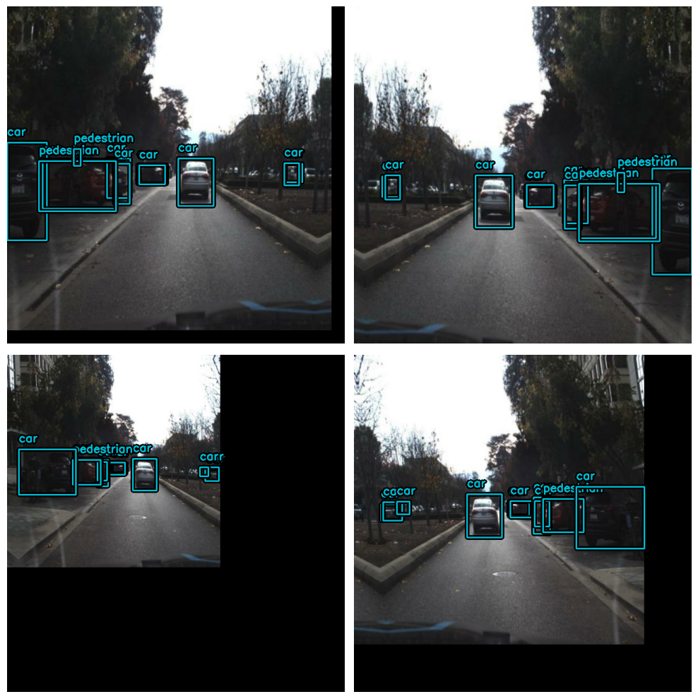
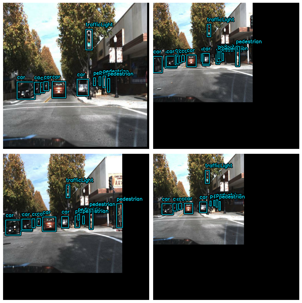
視覺化
def visualize_dataset(inputs, value_range, rows, cols, bounding_box_format):
    inputs = next(iter(inputs.take(1)))
    images, bounding_boxes = inputs["images"], inputs["bounding_boxes"]
    visualization.plot_bounding_box_gallery(
        images,
        value_range=value_range,
        rows=rows,
        cols=cols,
        y_true=bounding_boxes,
        scale=5,
        font_scale=0.7,
        bounding_box_format=bounding_box_format,
        class_mapping=class_mapping,
    )


visualize_dataset(
    train_ds, bounding_box_format="xyxy", value_range=(0, 255), rows=2, cols=2
)

visualize_dataset(
    val_ds, bounding_box_format="xyxy", value_range=(0, 255), rows=2, cols=2
)
我們需要從預處理字典中提取輸入,並準備好將其輸入到模型中。
def dict_to_tuple(inputs):
    return inputs["images"], inputs["bounding_boxes"]


train_ds = train_ds.map(dict_to_tuple, num_parallel_calls=tf.data.AUTOTUNE)
train_ds = train_ds.prefetch(tf.data.AUTOTUNE)

val_ds = val_ds.map(dict_to_tuple, num_parallel_calls=tf.data.AUTOTUNE)
val_ds = val_ds.prefetch(tf.data.AUTOTUNE)
建立模型
YOLOv8 是一種用於各種電腦視覺任務(例如物件偵測、影像分類和實例分割)的尖端 YOLO 模型。YOLOv5 的創建者 Ultralytics 也開發了 YOLOv8,與其前身相比,它在架構和開發人員體驗方面進行了許多改進和變更。YOLOv8 是最新的最先進模型,在業界備受推崇。
下表比較了五種不同大小(以像素為單位測量)的 YOLOv8 模型:YOLOv8n、YOLOv8s、YOLOv8m、YOLOv8l 和 YOLOv8x 的效能指標。這些指標包括驗證資料在不同交疊區域 (IoU) 閾值的平均精確度均值 (mAP) 值、使用 ONNX 格式在 CPU 上的推論速度和 A100 TensorRT、參數數量以及浮點運算次數 (FLOP)(分別以百萬和十億為單位)。隨著模型大小的增加,mAP、參數和 FLOP 通常會增加,而速度會降低。YOLOv8x 具有最高的 mAP、參數和 FLOP,但推論速度也最慢,而 YOLOv8n 具有最小的尺寸、最快的推論速度,以及最低的 mAP、參數和 FLOP。
| 模型 | 大小
(像素) | mAPval
50-95 | 速度
CPU ONNX
(毫秒) | 速度
A100 TensorRT
(毫秒) | 參數
(M) | FLOPs
(B) | | ------------------------------------------------------------------------------------ | --------------------- | -------------------- | ------------------------------ | ----------------------------------- | ------------------ | ----------------- | | YOLOv8n | 640 | 37.3 | 80.4 | 0.99 | 3.2 | 8.7 | | YOLOv8s | 640 | 44.9 | 128.4 | 1.20 | 11.2 | 28.6 | | YOLOv8m | 640 | 50.2 | 234.7 | 1.83 | 25.9 | 78.9 | | YOLOv8l | 640 | 52.9 | 375.2 | 2.39 | 43.7 | 165.2 | | YOLOv8x | 640 | 53.9 | 479.1 | 3.53 | 68.2 | 257.8 |
您可以在這篇 RoboFlow 部落格中閱讀更多有關 YOLOV8 及其架構的資訊
首先,我們將建立一個骨幹網路的實例,它將被我們的 yolov8 偵測器類別使用。
KerasCV 中提供的 YOLOV8 骨幹網路
- 不使用權重
1.   yolo_v8_xs_backbone
2.   yolo_v8_s_backbone
3.   yolo_v8_m_backbone
4.   yolo_v8_l_backbone
5.   yolo_v8_xl_backbone
- 使用預先訓練的 coco 權重
backbone = keras_cv.models.YOLOV8Backbone.from_preset(
    "yolo_v8_s_backbone_coco"  # We will use yolov8 small backbone with coco weights
)
1.   yolo_v8_xs_backbone_coco
2.   yolo_v8_s_backbone_coco
2.   yolo_v8_m_backbone_coco
2.   yolo_v8_l_backbone_coco
2.   yolo_v8_xl_backbone_coco

Downloading data from https://storage.googleapis.com/keras-cv/models/yolov8/coco/yolov8_s_backbone.h5
20596968/20596968 [==============================] - 0s 0us/step
接下來,讓我們使用 YOLOV8Detector 建立一個 YOLOV8 模型,該模型接受一個特徵提取器作為 backbone 引數、一個 num_classes 引數(指定要根據 class_mapping 列表的大小偵測的物件類別數量)、一個 bounding_box_format 引數(告知模型資料集中 bbox 的格式),最後,特徵金字塔網路 (FPN) 深度由 fpn_depth 引數指定。
由於 KerasCV,使用任何上述骨幹網路來建構 YOLOV8 非常簡單。
yolo = keras_cv.models.YOLOV8Detector(
    num_classes=len(class_mapping),
    bounding_box_format="xyxy",
    backbone=backbone,
    fpn_depth=1,
)
編譯模型
用於 YOLOV8 的損失
-
分類損失:此損失函數計算預期類別機率和實際類別機率之間的差異。在此例中,
binary_crossentropy是二元分類問題的著名解決方案。我們使用二元交叉熵,因為每個被識別出的東西都被分類為屬於或不屬於特定的物件類別(例如人、汽車等)。 -
框損失:
box_loss是用來衡量預測邊界框和真實值之間差異的損失函數。在此例中,使用完整 IoU (CIoU) 指標,它不僅衡量預測和真實邊界框之間的重疊,還會考慮長寬比、中心距離和框大小的差異。這些損失函數共同作用,透過最小化預測類別機率和邊界框與真實值之間的差異來最佳化物件偵測模型。
optimizer = tf.keras.optimizers.Adam(
    learning_rate=LEARNING_RATE,
    global_clipnorm=GLOBAL_CLIPNORM,
)

yolo.compile(
    optimizer=optimizer, classification_loss="binary_crossentropy", box_loss="ciou"
)
COCO 指標回呼
我們將使用 KerasCV 的 BoxCOCOMetrics 來評估模型並計算 Map(平均精確度均值)分數、召回率和精確度。當 mAP 分數提高時,我們也會儲存模型。
class EvaluateCOCOMetricsCallback(keras.callbacks.Callback):
    def __init__(self, data, save_path):
        super().__init__()
        self.data = data
        self.metrics = keras_cv.metrics.BoxCOCOMetrics(
            bounding_box_format="xyxy",
            evaluate_freq=1e9,
        )

        self.save_path = save_path
        self.best_map = -1.0

    def on_epoch_end(self, epoch, logs):
        self.metrics.reset_state()
        for batch in self.data:
            images, y_true = batch[0], batch[1]
            y_pred = self.model.predict(images, verbose=0)
            self.metrics.update_state(y_true, y_pred)

        metrics = self.metrics.result(force=True)
        logs.update(metrics)

        current_map = metrics["MaP"]
        if current_map > self.best_map:
            self.best_map = current_map
            self.model.save(self.save_path)  # Save the model when mAP improves

        return logs
訓練模型
yolo.fit(
    train_ds,
    validation_data=val_ds,
    epochs=3,
    callbacks=[EvaluateCOCOMetricsCallback(val_ds, "model.h5")],
)
Epoch 1/3
1463/1463 [==============================] - 633s 390ms/step - loss: 10.1535 - box_loss: 2.5659 - class_loss: 7.5876 - val_loss: 3.9852 - val_box_loss: 3.1973 - val_class_loss: 0.7879 - MaP: 0.0095 - MaP@[IoU=50]: 0.0193 - MaP@[IoU=75]: 0.0074 - MaP@[area=small]: 0.0021 - MaP@[area=medium]: 0.0164 - MaP@[area=large]: 0.0010 - Recall@[max_detections=1]: 0.0096 - Recall@[max_detections=10]: 0.0160 - Recall@[max_detections=100]: 0.0160 - Recall@[area=small]: 0.0034 - Recall@[area=medium]: 0.0283 - Recall@[area=large]: 0.0010
Epoch 2/3
1463/1463 [==============================] - 554s 378ms/step - loss: 2.6961 - box_loss: 2.2861 - class_loss: 0.4100 - val_loss: 3.8292 - val_box_loss: 3.0052 - val_class_loss: 0.8240 - MaP: 0.0077 - MaP@[IoU=50]: 0.0197 - MaP@[IoU=75]: 0.0043 - MaP@[area=small]: 0.0075 - MaP@[area=medium]: 0.0126 - MaP@[area=large]: 0.0050 - Recall@[max_detections=1]: 0.0088 - Recall@[max_detections=10]: 0.0154 - Recall@[max_detections=100]: 0.0154 - Recall@[area=small]: 0.0075 - Recall@[area=medium]: 0.0191 - Recall@[area=large]: 0.0280
Epoch 3/3
1463/1463 [==============================] - 558s 381ms/step - loss: 2.5930 - box_loss: 2.2018 - class_loss: 0.3912 - val_loss: 3.4796 - val_box_loss: 2.8472 - val_class_loss: 0.6323 - MaP: 0.0145 - MaP@[IoU=50]: 0.0398 - MaP@[IoU=75]: 0.0072 - MaP@[area=small]: 0.0077 - MaP@[area=medium]: 0.0227 - MaP@[area=large]: 0.0079 - Recall@[max_detections=1]: 0.0120 - Recall@[max_detections=10]: 0.0257 - Recall@[max_detections=100]: 0.0258 - Recall@[area=small]: 0.0093 - Recall@[area=medium]: 0.0396 - Recall@[area=large]: 0.0226

<keras.callbacks.History at 0x7f3e01ca6d70>
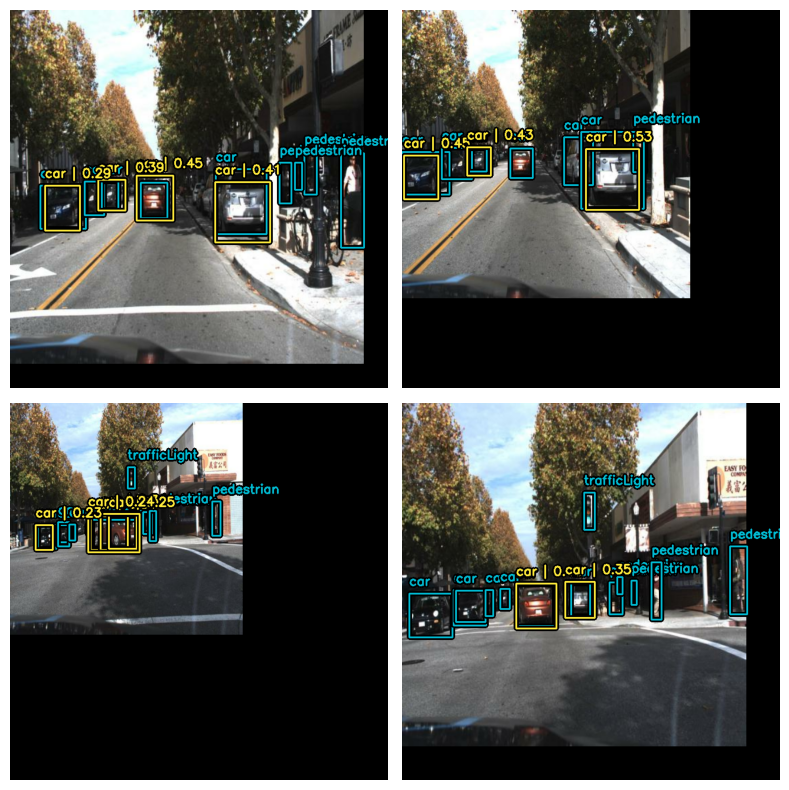
視覺化預測
def visualize_detections(model, dataset, bounding_box_format):
    images, y_true = next(iter(dataset.take(1)))
    y_pred = model.predict(images)
    y_pred = bounding_box.to_ragged(y_pred)
    visualization.plot_bounding_box_gallery(
        images,
        value_range=(0, 255),
        bounding_box_format=bounding_box_format,
        y_true=y_true,
        y_pred=y_pred,
        scale=4,
        rows=2,
        cols=2,
        show=True,
        font_scale=0.7,
        class_mapping=class_mapping,
    )


visualize_detections(yolo, dataset=val_ds, bounding_box_format="xyxy")
1/1 [==============================] - 0s 115ms/step