函式式 API
作者: fchollet
建立日期 2019/03/01
上次修改日期 2023/06/25
說明: 函式式 API 的完整指南。

設定
import numpy as np
import keras
from keras import layers
from keras import ops
簡介
Keras 的函式式 API 是一種建立比 keras.Sequential API 更具彈性的模型的方法。函式式 API 可以處理具有非線性拓撲、共享層,甚至多個輸入或輸出的模型。
主要概念是,深度學習模型通常是層的有向無環圖 (DAG)。因此,函式式 API 是一種建立層圖的方法。
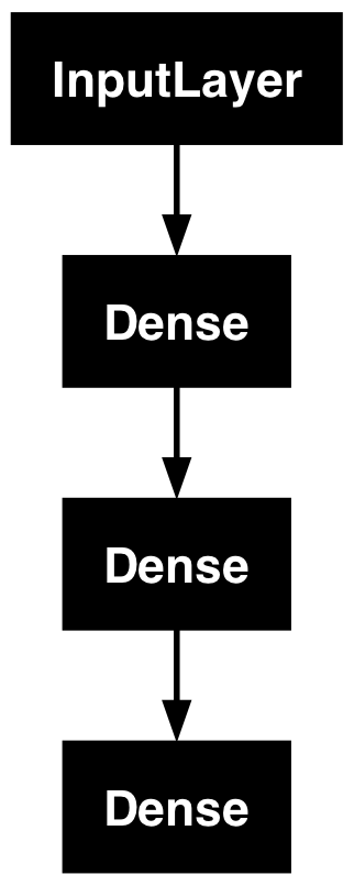
考慮以下模型
(input: 784-dimensional vectors)
       ↧
[Dense (64 units, relu activation)]
       ↧
[Dense (64 units, relu activation)]
       ↧
[Dense (10 units, softmax activation)]
       ↧
(output: logits of a probability distribution over 10 classes)
這是一個具有三層的基本圖。若要使用函式式 API 建立此模型,請從建立輸入節點開始
inputs = keras.Input(shape=(784,))
資料的形狀設定為 784 維向量。批次大小始終省略,因為僅指定每個樣本的形狀。
例如,如果您有一個形狀為 (32, 32, 3) 的圖像輸入,您會使用
# Just for demonstration purposes.
img_inputs = keras.Input(shape=(32, 32, 3))
傳回的 inputs 包含您饋送到模型的輸入資料的形狀和 dtype 的相關資訊。這是形狀
inputs.shape
(None, 784)
這是 dtype
inputs.dtype
'float32'
您藉由在這個 inputs 物件上呼叫一個層來建立層圖中的新節點
dense = layers.Dense(64, activation="relu")
x = dense(inputs)
「層呼叫」動作就像是從「inputs」到您建立的此層繪製箭頭。您正在將輸入「傳遞」到 dense 層,並且您會取得 x 作為輸出。
讓我們在層圖中新增更多層
x = layers.Dense(64, activation="relu")(x)
outputs = layers.Dense(10)(x)
此時,您可以藉由在層圖中指定其輸入和輸出來建立 Model
model = keras.Model(inputs=inputs, outputs=outputs, name="mnist_model")
讓我們看看模型摘要的外觀
model.summary()
Model: "mnist_model"
┏━━━━━━━━━━━━━━━━━━━━━━━━━━━━━━━━━┳━━━━━━━━━━━━━━━━━━━━━━━━┳━━━━━━━━━━━━━━━┓
┃ Layer (type)                    ┃ Output Shape           ┃       Param # ┃
┡━━━━━━━━━━━━━━━━━━━━━━━━━━━━━━━━━╇━━━━━━━━━━━━━━━━━━━━━━━━╇━━━━━━━━━━━━━━━┩
│ input_layer (InputLayer)        │ (None, 784)            │             0 │
├─────────────────────────────────┼────────────────────────┼───────────────┤
│ dense (Dense)                   │ (None, 64)             │        50,240 │
├─────────────────────────────────┼────────────────────────┼───────────────┤
│ dense_1 (Dense)                 │ (None, 64)             │         4,160 │
├─────────────────────────────────┼────────────────────────┼───────────────┤
│ dense_2 (Dense)                 │ (None, 10)             │           650 │
└─────────────────────────────────┴────────────────────────┴───────────────┘
Total params: 55,050 (215.04 KB)
Trainable params: 55,050 (215.04 KB)
Non-trainable params: 0 (0.00 B)
您也可以將模型繪製為圖形
keras.utils.plot_model(model, "my_first_model.png")
並且,可選擇性地,在繪製的圖形中顯示每個層的輸入和輸出形狀
keras.utils.plot_model(model, "my_first_model_with_shape_info.png", show_shapes=True)
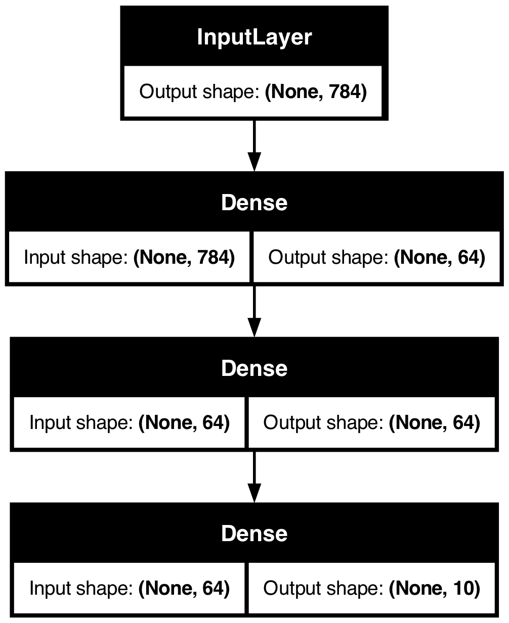
此圖和程式碼幾乎相同。在程式碼版本中,連線箭頭由呼叫運算取代。
「層圖」是深度學習模型的直觀心智圖像,而函式式 API 是一種建立與此密切相符的模型的方法。
訓練、評估和推論
對於使用函式式 API 建立的模型,訓練、評估和推論的工作方式與 Sequential 模型完全相同。
Model 類別提供內建的訓練迴圈 (fit() 方法) 和內建的評估迴圈 (evaluate() 方法)。請注意,您可以輕鬆自訂這些迴圈以實作您自己的訓練常式。另請參閱有關自訂 fit() 中發生情況的指南
在此,載入 MNIST 影像資料,將其重新塑形為向量,將模型擬合到資料上 (同時監控驗證分割上的效能),然後評估測試資料上的模型
(x_train, y_train), (x_test, y_test) = keras.datasets.mnist.load_data()

x_train = x_train.reshape(60000, 784).astype("float32") / 255
x_test = x_test.reshape(10000, 784).astype("float32") / 255

model.compile(
    loss=keras.losses.SparseCategoricalCrossentropy(from_logits=True),
    optimizer=keras.optimizers.RMSprop(),
    metrics=["accuracy"],
)

history = model.fit(x_train, y_train, batch_size=64, epochs=2, validation_split=0.2)

test_scores = model.evaluate(x_test, y_test, verbose=2)
print("Test loss:", test_scores[0])
print("Test accuracy:", test_scores[1])
Epoch 1/2
 750/750 ━━━━━━━━━━━━━━━━━━━━ 1s 863us/step - accuracy: 0.8425 - loss: 0.5733 - val_accuracy: 0.9496 - val_loss: 0.1711
Epoch 2/2
 750/750 ━━━━━━━━━━━━━━━━━━━━ 1s 859us/step - accuracy: 0.9509 - loss: 0.1641 - val_accuracy: 0.9578 - val_loss: 0.1396
313/313 - 0s - 341us/step - accuracy: 0.9613 - loss: 0.1288
Test loss: 0.12876172363758087
Test accuracy: 0.9613000154495239
如需進一步閱讀,請參閱訓練和評估指南。
儲存和序列化
對於使用函式式 API 建立的模型,儲存模型和序列化的工作方式與 Sequential 模型相同。儲存函式式模型的標準方法是呼叫 model.save() 將整個模型儲存為單一檔案。您稍後可以從此檔案重新建立相同的模型,即使建立模型的程式碼不再可用。
此已儲存的檔案包含:- 模型架構 - 模型權重值 (在訓練期間學習到的) - 模型訓練組態 (如果有) (傳遞至 compile()) - 優化器及其狀態 (如果有) (從您停止的地方重新啟動訓練)
model.save("my_model.keras")
del model
# Recreate the exact same model purely from the file:
model = keras.models.load_model("my_model.keras")
如需詳細資訊,請閱讀模型序列化和儲存指南。
使用相同的層圖來定義多個模型
在函式式 API 中,模型是藉由在層圖中指定其輸入和輸出來建立的。這表示單一層圖可以用來產生多個模型。
在以下範例中,您使用相同的層堆疊來實例化兩個模型:一個將影像輸入轉換為 16 維向量的 encoder 模型,以及一個用於訓練的端對端 autoencoder 模型。
encoder_input = keras.Input(shape=(28, 28, 1), name="img")
x = layers.Conv2D(16, 3, activation="relu")(encoder_input)
x = layers.Conv2D(32, 3, activation="relu")(x)
x = layers.MaxPooling2D(3)(x)
x = layers.Conv2D(32, 3, activation="relu")(x)
x = layers.Conv2D(16, 3, activation="relu")(x)
encoder_output = layers.GlobalMaxPooling2D()(x)

encoder = keras.Model(encoder_input, encoder_output, name="encoder")
encoder.summary()

x = layers.Reshape((4, 4, 1))(encoder_output)
x = layers.Conv2DTranspose(16, 3, activation="relu")(x)
x = layers.Conv2DTranspose(32, 3, activation="relu")(x)
x = layers.UpSampling2D(3)(x)
x = layers.Conv2DTranspose(16, 3, activation="relu")(x)
decoder_output = layers.Conv2DTranspose(1, 3, activation="relu")(x)

autoencoder = keras.Model(encoder_input, decoder_output, name="autoencoder")
autoencoder.summary()
Model: "encoder"
┏━━━━━━━━━━━━━━━━━━━━━━━━━━━━━━━━━┳━━━━━━━━━━━━━━━━━━━━━━━━┳━━━━━━━━━━━━━━━┓
┃ Layer (type)                    ┃ Output Shape           ┃       Param # ┃
┡━━━━━━━━━━━━━━━━━━━━━━━━━━━━━━━━━╇━━━━━━━━━━━━━━━━━━━━━━━━╇━━━━━━━━━━━━━━━┩
│ img (InputLayer)                │ (None, 28, 28, 1)      │             0 │
├─────────────────────────────────┼────────────────────────┼───────────────┤
│ conv2d (Conv2D)                 │ (None, 26, 26, 16)     │           160 │
├─────────────────────────────────┼────────────────────────┼───────────────┤
│ conv2d_1 (Conv2D)               │ (None, 24, 24, 32)     │         4,640 │
├─────────────────────────────────┼────────────────────────┼───────────────┤
│ max_pooling2d (MaxPooling2D)    │ (None, 8, 8, 32)       │             0 │
├─────────────────────────────────┼────────────────────────┼───────────────┤
│ conv2d_2 (Conv2D)               │ (None, 6, 6, 32)       │         9,248 │
├─────────────────────────────────┼────────────────────────┼───────────────┤
│ conv2d_3 (Conv2D)               │ (None, 4, 4, 16)       │         4,624 │
├─────────────────────────────────┼────────────────────────┼───────────────┤
│ global_max_pooling2d            │ (None, 16)             │             0 │
│ (GlobalMaxPooling2D)            │                        │               │
└─────────────────────────────────┴────────────────────────┴───────────────┘
Total params: 18,672 (72.94 KB)
Trainable params: 18,672 (72.94 KB)
Non-trainable params: 0 (0.00 B)
Model: "autoencoder"
┏━━━━━━━━━━━━━━━━━━━━━━━━━━━━━━━━━┳━━━━━━━━━━━━━━━━━━━━━━━━┳━━━━━━━━━━━━━━━┓
┃ Layer (type)                    ┃ Output Shape           ┃       Param # ┃
┡━━━━━━━━━━━━━━━━━━━━━━━━━━━━━━━━━╇━━━━━━━━━━━━━━━━━━━━━━━━╇━━━━━━━━━━━━━━━┩
│ img (InputLayer)                │ (None, 28, 28, 1)      │             0 │
├─────────────────────────────────┼────────────────────────┼───────────────┤
│ conv2d (Conv2D)                 │ (None, 26, 26, 16)     │           160 │
├─────────────────────────────────┼────────────────────────┼───────────────┤
│ conv2d_1 (Conv2D)               │ (None, 24, 24, 32)     │         4,640 │
├─────────────────────────────────┼────────────────────────┼───────────────┤
│ max_pooling2d (MaxPooling2D)    │ (None, 8, 8, 32)       │             0 │
├─────────────────────────────────┼────────────────────────┼───────────────┤
│ conv2d_2 (Conv2D)               │ (None, 6, 6, 32)       │         9,248 │
├─────────────────────────────────┼────────────────────────┼───────────────┤
│ conv2d_3 (Conv2D)               │ (None, 4, 4, 16)       │         4,624 │
├─────────────────────────────────┼────────────────────────┼───────────────┤
│ global_max_pooling2d            │ (None, 16)             │             0 │
│ (GlobalMaxPooling2D)            │                        │               │
├─────────────────────────────────┼────────────────────────┼───────────────┤
│ reshape (Reshape)               │ (None, 4, 4, 1)        │             0 │
├─────────────────────────────────┼────────────────────────┼───────────────┤
│ conv2d_transpose                │ (None, 6, 6, 16)       │           160 │
│ (Conv2DTranspose)               │                        │               │
├─────────────────────────────────┼────────────────────────┼───────────────┤
│ conv2d_transpose_1              │ (None, 8, 8, 32)       │         4,640 │
│ (Conv2DTranspose)               │                        │               │
├─────────────────────────────────┼────────────────────────┼───────────────┤
│ up_sampling2d (UpSampling2D)    │ (None, 24, 24, 32)     │             0 │
├─────────────────────────────────┼────────────────────────┼───────────────┤
│ conv2d_transpose_2              │ (None, 26, 26, 16)     │         4,624 │
│ (Conv2DTranspose)               │                        │               │
├─────────────────────────────────┼────────────────────────┼───────────────┤
│ conv2d_transpose_3              │ (None, 28, 28, 1)      │           145 │
│ (Conv2DTranspose)               │                        │               │
└─────────────────────────────────┴────────────────────────┴───────────────┘
Total params: 28,241 (110.32 KB)
Trainable params: 28,241 (110.32 KB)
Non-trainable params: 0 (0.00 B)
在此,解碼架構與編碼架構完全對稱,因此輸出形狀與輸入形狀 (28, 28, 1) 相同。
Conv2D 層的反向是 Conv2DTranspose 層,而 MaxPooling2D 層的反向是 UpSampling2D 層。
所有模型都是可呼叫的,就像層一樣
您可以將任何模型視為層,方法是在 Input 上或在另一層的輸出上調用它。藉由呼叫模型,您不僅重複使用模型的架構,您也重複使用其權重。
若要查看此功能的運作方式,這裡有一個自動編碼器範例的不同做法,其中會建立一個編碼器模型、一個解碼器模型,並將它們鏈結在兩個呼叫中以取得自動編碼器模型
encoder_input = keras.Input(shape=(28, 28, 1), name="original_img")
x = layers.Conv2D(16, 3, activation="relu")(encoder_input)
x = layers.Conv2D(32, 3, activation="relu")(x)
x = layers.MaxPooling2D(3)(x)
x = layers.Conv2D(32, 3, activation="relu")(x)
x = layers.Conv2D(16, 3, activation="relu")(x)
encoder_output = layers.GlobalMaxPooling2D()(x)

encoder = keras.Model(encoder_input, encoder_output, name="encoder")
encoder.summary()

decoder_input = keras.Input(shape=(16,), name="encoded_img")
x = layers.Reshape((4, 4, 1))(decoder_input)
x = layers.Conv2DTranspose(16, 3, activation="relu")(x)
x = layers.Conv2DTranspose(32, 3, activation="relu")(x)
x = layers.UpSampling2D(3)(x)
x = layers.Conv2DTranspose(16, 3, activation="relu")(x)
decoder_output = layers.Conv2DTranspose(1, 3, activation="relu")(x)

decoder = keras.Model(decoder_input, decoder_output, name="decoder")
decoder.summary()

autoencoder_input = keras.Input(shape=(28, 28, 1), name="img")
encoded_img = encoder(autoencoder_input)
decoded_img = decoder(encoded_img)
autoencoder = keras.Model(autoencoder_input, decoded_img, name="autoencoder")
autoencoder.summary()
Model: "encoder"
┏━━━━━━━━━━━━━━━━━━━━━━━━━━━━━━━━━┳━━━━━━━━━━━━━━━━━━━━━━━━┳━━━━━━━━━━━━━━━┓
┃ Layer (type)                    ┃ Output Shape           ┃       Param # ┃
┡━━━━━━━━━━━━━━━━━━━━━━━━━━━━━━━━━╇━━━━━━━━━━━━━━━━━━━━━━━━╇━━━━━━━━━━━━━━━┩
│ original_img (InputLayer)       │ (None, 28, 28, 1)      │             0 │
├─────────────────────────────────┼────────────────────────┼───────────────┤
│ conv2d_4 (Conv2D)               │ (None, 26, 26, 16)     │           160 │
├─────────────────────────────────┼────────────────────────┼───────────────┤
│ conv2d_5 (Conv2D)               │ (None, 24, 24, 32)     │         4,640 │
├─────────────────────────────────┼────────────────────────┼───────────────┤
│ max_pooling2d_1 (MaxPooling2D)  │ (None, 8, 8, 32)       │             0 │
├─────────────────────────────────┼────────────────────────┼───────────────┤
│ conv2d_6 (Conv2D)               │ (None, 6, 6, 32)       │         9,248 │
├─────────────────────────────────┼────────────────────────┼───────────────┤
│ conv2d_7 (Conv2D)               │ (None, 4, 4, 16)       │         4,624 │
├─────────────────────────────────┼────────────────────────┼───────────────┤
│ global_max_pooling2d_1          │ (None, 16)             │             0 │
│ (GlobalMaxPooling2D)            │                        │               │
└─────────────────────────────────┴────────────────────────┴───────────────┘
Total params: 18,672 (72.94 KB)
Trainable params: 18,672 (72.94 KB)
Non-trainable params: 0 (0.00 B)
Model: "decoder"
┏━━━━━━━━━━━━━━━━━━━━━━━━━━━━━━━━━┳━━━━━━━━━━━━━━━━━━━━━━━━┳━━━━━━━━━━━━━━━┓
┃ Layer (type)                    ┃ Output Shape           ┃       Param # ┃
┡━━━━━━━━━━━━━━━━━━━━━━━━━━━━━━━━━╇━━━━━━━━━━━━━━━━━━━━━━━━╇━━━━━━━━━━━━━━━┩
│ encoded_img (InputLayer)        │ (None, 16)             │             0 │
├─────────────────────────────────┼────────────────────────┼───────────────┤
│ reshape_1 (Reshape)             │ (None, 4, 4, 1)        │             0 │
├─────────────────────────────────┼────────────────────────┼───────────────┤
│ conv2d_transpose_4              │ (None, 6, 6, 16)       │           160 │
│ (Conv2DTranspose)               │                        │               │
├─────────────────────────────────┼────────────────────────┼───────────────┤
│ conv2d_transpose_5              │ (None, 8, 8, 32)       │         4,640 │
│ (Conv2DTranspose)               │                        │               │
├─────────────────────────────────┼────────────────────────┼───────────────┤
│ up_sampling2d_1 (UpSampling2D)  │ (None, 24, 24, 32)     │             0 │
├─────────────────────────────────┼────────────────────────┼───────────────┤
│ conv2d_transpose_6              │ (None, 26, 26, 16)     │         4,624 │
│ (Conv2DTranspose)               │                        │               │
├─────────────────────────────────┼────────────────────────┼───────────────┤
│ conv2d_transpose_7              │ (None, 28, 28, 1)      │           145 │
│ (Conv2DTranspose)               │                        │               │
└─────────────────────────────────┴────────────────────────┴───────────────┘
Total params: 9,569 (37.38 KB)
Trainable params: 9,569 (37.38 KB)
Non-trainable params: 0 (0.00 B)
Model: "autoencoder"
┏━━━━━━━━━━━━━━━━━━━━━━━━━━━━━━━━━┳━━━━━━━━━━━━━━━━━━━━━━━━┳━━━━━━━━━━━━━━━┓
┃ Layer (type)                    ┃ Output Shape           ┃       Param # ┃
┡━━━━━━━━━━━━━━━━━━━━━━━━━━━━━━━━━╇━━━━━━━━━━━━━━━━━━━━━━━━╇━━━━━━━━━━━━━━━┩
│ img (InputLayer)                │ (None, 28, 28, 1)      │             0 │
├─────────────────────────────────┼────────────────────────┼───────────────┤
│ encoder (Functional)            │ (None, 16)             │        18,672 │
├─────────────────────────────────┼────────────────────────┼───────────────┤
│ decoder (Functional)            │ (None, 28, 28, 1)      │         9,569 │
└─────────────────────────────────┴────────────────────────┴───────────────┘
Total params: 28,241 (110.32 KB)
Trainable params: 28,241 (110.32 KB)
Non-trainable params: 0 (0.00 B)
如您所見,模型可以巢狀:模型可以包含子模型 (因為模型就像層一樣)。模型巢狀的常見使用案例是集成。例如,以下是如何將一組模型集成到一個模型中,該模型會平均它們的預測
def get_model():
    inputs = keras.Input(shape=(128,))
    outputs = layers.Dense(1)(inputs)
    return keras.Model(inputs, outputs)


model1 = get_model()
model2 = get_model()
model3 = get_model()

inputs = keras.Input(shape=(128,))
y1 = model1(inputs)
y2 = model2(inputs)
y3 = model3(inputs)
outputs = layers.average([y1, y2, y3])
ensemble_model = keras.Model(inputs=inputs, outputs=outputs)
操縱複雜的圖形拓撲
具有多個輸入和輸出的模型
函式式 API 可輕鬆操控多個輸入和輸出。這無法使用 Sequential API 處理。
例如,如果您正在建立一個系統,用於根據優先順序排列客戶問題單,並將其路由到正確的部門,則模型將具有三個輸入
- 問題單的標題 (文字輸入),
- 問題單的文字主體 (文字輸入),以及
- 使用者新增的任何標籤 (類別輸入)
此模型將具有兩個輸出
- 介於 0 和 1 之間的優先順序分數 (純量 sigmoid 輸出),以及
- 應該處理問題單的部門 (在部門集合上的 softmax 輸出)。
您可以使用函式式 API 以幾行程式碼建立此模型
num_tags = 12  # Number of unique issue tags
num_words = 10000  # Size of vocabulary obtained when preprocessing text data
num_departments = 4  # Number of departments for predictions

title_input = keras.Input(
    shape=(None,), name="title"
)  # Variable-length sequence of ints
body_input = keras.Input(shape=(None,), name="body")  # Variable-length sequence of ints
tags_input = keras.Input(
    shape=(num_tags,), name="tags"
)  # Binary vectors of size `num_tags`

# Embed each word in the title into a 64-dimensional vector
title_features = layers.Embedding(num_words, 64)(title_input)
# Embed each word in the text into a 64-dimensional vector
body_features = layers.Embedding(num_words, 64)(body_input)

# Reduce sequence of embedded words in the title into a single 128-dimensional vector
title_features = layers.LSTM(128)(title_features)
# Reduce sequence of embedded words in the body into a single 32-dimensional vector
body_features = layers.LSTM(32)(body_features)

# Merge all available features into a single large vector via concatenation
x = layers.concatenate([title_features, body_features, tags_input])

# Stick a logistic regression for priority prediction on top of the features
priority_pred = layers.Dense(1, name="priority")(x)
# Stick a department classifier on top of the features
department_pred = layers.Dense(num_departments, name="department")(x)

# Instantiate an end-to-end model predicting both priority and department
model = keras.Model(
    inputs=[title_input, body_input, tags_input],
    outputs={"priority": priority_pred, "department": department_pred},
)
現在繪製模型
keras.utils.plot_model(model, "multi_input_and_output_model.png", show_shapes=True)

在編譯此模型時,您可以為每個輸出指派不同的損失。您甚至可以為每個損失指派不同的權重 – 以調整它們對總訓練損失的貢獻。
model.compile(
    optimizer=keras.optimizers.RMSprop(1e-3),
    loss=[
        keras.losses.BinaryCrossentropy(from_logits=True),
        keras.losses.CategoricalCrossentropy(from_logits=True),
    ],
    loss_weights=[1.0, 0.2],
)
由於輸出層具有不同的名稱,您也可以使用對應的層名稱指定損失和損失權重
model.compile(
    optimizer=keras.optimizers.RMSprop(1e-3),
    loss={
        "priority": keras.losses.BinaryCrossentropy(from_logits=True),
        "department": keras.losses.CategoricalCrossentropy(from_logits=True),
    },
    loss_weights={"priority": 1.0, "department": 0.2},
)
藉由傳遞 NumPy 輸入和目標陣列的清單來訓練模型
# Dummy input data
title_data = np.random.randint(num_words, size=(1280, 12))
body_data = np.random.randint(num_words, size=(1280, 100))
tags_data = np.random.randint(2, size=(1280, num_tags)).astype("float32")

# Dummy target data
priority_targets = np.random.random(size=(1280, 1))
dept_targets = np.random.randint(2, size=(1280, num_departments))

model.fit(
    {"title": title_data, "body": body_data, "tags": tags_data},
    {"priority": priority_targets, "department": dept_targets},
    epochs=2,
    batch_size=32,
)
Epoch 1/2
 40/40 ━━━━━━━━━━━━━━━━━━━━ 3s 57ms/step - loss: 1108.3792
Epoch 2/2
 40/40 ━━━━━━━━━━━━━━━━━━━━ 2s 54ms/step - loss: 621.3049

<keras.src.callbacks.history.History at 0x34afc3d90>
當使用 Dataset 物件呼叫 fit 時,它應該產生類似 ([title_data, body_data, tags_data], [priority_targets, dept_targets]) 的清單元組,或類似 ({'title': title_data, 'body': body_data, 'tags': tags_data}, {'priority': priority_targets, 'department': dept_targets}) 的字典元組。
如需更詳細的說明,請參閱訓練和評估指南。
玩具 ResNet 模型
除了具有多個輸入和輸出的模型之外,函式式 API 還可以輕鬆操控非線性連線拓撲 – 這些是具有未依序連線的層的模型,這是 Sequential API 無法處理的。
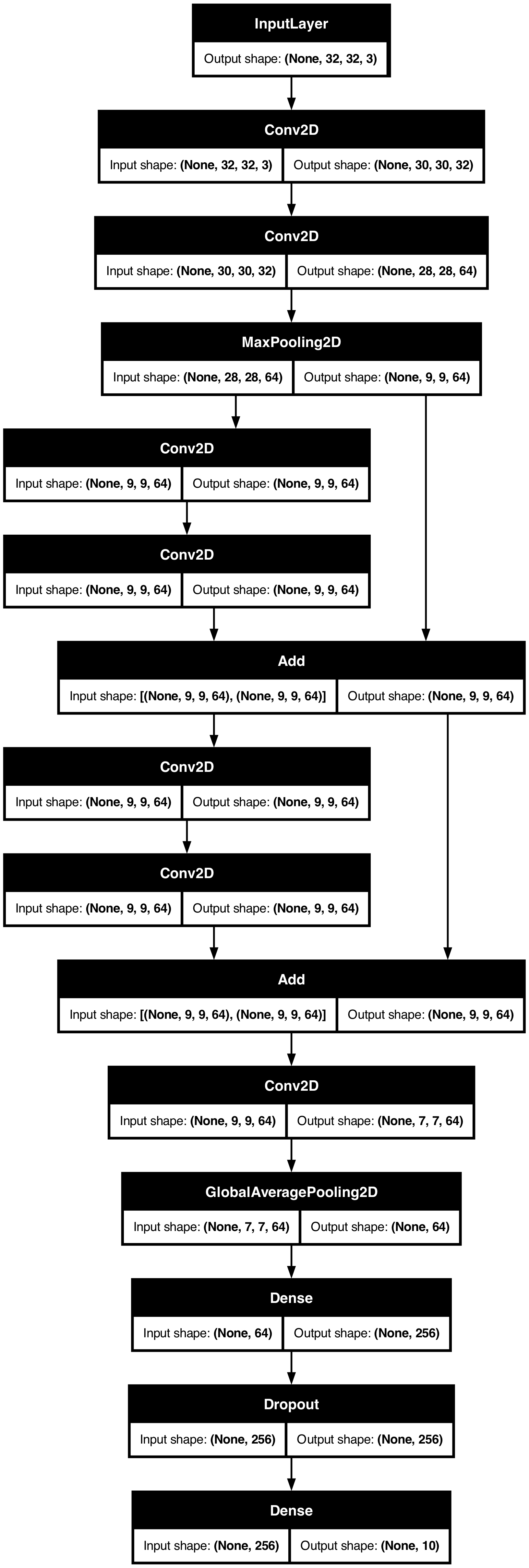
其常見使用案例是殘差連線。讓我們為 CIFAR10 建立一個玩具 ResNet 模型來示範這一點
inputs = keras.Input(shape=(32, 32, 3), name="img")
x = layers.Conv2D(32, 3, activation="relu")(inputs)
x = layers.Conv2D(64, 3, activation="relu")(x)
block_1_output = layers.MaxPooling2D(3)(x)

x = layers.Conv2D(64, 3, activation="relu", padding="same")(block_1_output)
x = layers.Conv2D(64, 3, activation="relu", padding="same")(x)
block_2_output = layers.add([x, block_1_output])

x = layers.Conv2D(64, 3, activation="relu", padding="same")(block_2_output)
x = layers.Conv2D(64, 3, activation="relu", padding="same")(x)
block_3_output = layers.add([x, block_2_output])

x = layers.Conv2D(64, 3, activation="relu")(block_3_output)
x = layers.GlobalAveragePooling2D()(x)
x = layers.Dense(256, activation="relu")(x)
x = layers.Dropout(0.5)(x)
outputs = layers.Dense(10)(x)

model = keras.Model(inputs, outputs, name="toy_resnet")
model.summary()
Model: "toy_resnet"
┏━━━━━━━━━━━━━━━━━━━━━┳━━━━━━━━━━━━━━━━━━━┳━━━━━━━━━━━━┳━━━━━━━━━━━━━━━━━━━┓
┃ Layer (type)        ┃ Output Shape      ┃    Param # ┃ Connected to      ┃
┡━━━━━━━━━━━━━━━━━━━━━╇━━━━━━━━━━━━━━━━━━━╇━━━━━━━━━━━━╇━━━━━━━━━━━━━━━━━━━┩
│ img (InputLayer)    │ (None, 32, 32, 3) │          0 │ -                 │
├─────────────────────┼───────────────────┼────────────┼───────────────────┤
│ conv2d_8 (Conv2D)   │ (None, 30, 30,    │        896 │ img[0][0]         │
│                     │ 32)               │            │                   │
├─────────────────────┼───────────────────┼────────────┼───────────────────┤
│ conv2d_9 (Conv2D)   │ (None, 28, 28,    │     18,496 │ conv2d_8[0][0]    │
│                     │ 64)               │            │                   │
├─────────────────────┼───────────────────┼────────────┼───────────────────┤
│ max_pooling2d_2     │ (None, 9, 9, 64)  │          0 │ conv2d_9[0][0]    │
│ (MaxPooling2D)      │                   │            │                   │
├─────────────────────┼───────────────────┼────────────┼───────────────────┤
│ conv2d_10 (Conv2D)  │ (None, 9, 9, 64)  │     36,928 │ max_pooling2d_2[… │
├─────────────────────┼───────────────────┼────────────┼───────────────────┤
│ conv2d_11 (Conv2D)  │ (None, 9, 9, 64)  │     36,928 │ conv2d_10[0][0]   │
├─────────────────────┼───────────────────┼────────────┼───────────────────┤
│ add (Add)           │ (None, 9, 9, 64)  │          0 │ conv2d_11[0][0],  │
│                     │                   │            │ max_pooling2d_2[… │
├─────────────────────┼───────────────────┼────────────┼───────────────────┤
│ conv2d_12 (Conv2D)  │ (None, 9, 9, 64)  │     36,928 │ add[0][0]         │
├─────────────────────┼───────────────────┼────────────┼───────────────────┤
│ conv2d_13 (Conv2D)  │ (None, 9, 9, 64)  │     36,928 │ conv2d_12[0][0]   │
├─────────────────────┼───────────────────┼────────────┼───────────────────┤
│ add_1 (Add)         │ (None, 9, 9, 64)  │          0 │ conv2d_13[0][0],  │
│                     │                   │            │ add[0][0]         │
├─────────────────────┼───────────────────┼────────────┼───────────────────┤
│ conv2d_14 (Conv2D)  │ (None, 7, 7, 64)  │     36,928 │ add_1[0][0]       │
├─────────────────────┼───────────────────┼────────────┼───────────────────┤
│ global_average_poo… │ (None, 64)        │          0 │ conv2d_14[0][0]   │
│ (GlobalAveragePool… │                   │            │                   │
├─────────────────────┼───────────────────┼────────────┼───────────────────┤
│ dense_6 (Dense)     │ (None, 256)       │     16,640 │ global_average_p… │
├─────────────────────┼───────────────────┼────────────┼───────────────────┤
│ dropout (Dropout)   │ (None, 256)       │          0 │ dense_6[0][0]     │
├─────────────────────┼───────────────────┼────────────┼───────────────────┤
│ dense_7 (Dense)     │ (None, 10)        │      2,570 │ dropout[0][0]     │
└─────────────────────┴───────────────────┴────────────┴───────────────────┘
Total params: 223,242 (872.04 KB)
Trainable params: 223,242 (872.04 KB)
Non-trainable params: 0 (0.00 B)
繪製模型
keras.utils.plot_model(model, "mini_resnet.png", show_shapes=True)
現在訓練模型
(x_train, y_train), (x_test, y_test) = keras.datasets.cifar10.load_data()

x_train = x_train.astype("float32") / 255.0
x_test = x_test.astype("float32") / 255.0
y_train = keras.utils.to_categorical(y_train, 10)
y_test = keras.utils.to_categorical(y_test, 10)

model.compile(
    optimizer=keras.optimizers.RMSprop(1e-3),
    loss=keras.losses.CategoricalCrossentropy(from_logits=True),
    metrics=["acc"],
)
# We restrict the data to the first 1000 samples so as to limit execution time
# on Colab. Try to train on the entire dataset until convergence!
model.fit(
    x_train[:1000],
    y_train[:1000],
    batch_size=64,
    epochs=1,
    validation_split=0.2,
)
 13/13 ━━━━━━━━━━━━━━━━━━━━ 1s 60ms/step - acc: 0.1096 - loss: 2.3053 - val_acc: 0.1150 - val_loss: 2.2973

<keras.src.callbacks.history.History at 0x1758bed40>
共用層
功能式 API 的另一個優點是用於使用共享層的模型。共享層是層的實例,在同一個模型中被多次重複使用 — 它們學習對應於層圖中多個路徑的特徵。
共享層通常用於編碼來自相似空間的輸入(例如,兩個具有相似詞彙的不同文本片段)。它們能夠在這些不同的輸入之間共享資訊,並且使模型能夠在較少的數據上進行訓練。如果一個詞出現在其中一個輸入中,那麼將會使所有經過共享層的輸入處理受益。
要在功能式 API 中共享一個層,請多次呼叫同一個層實例。例如,這是一個在兩個不同文字輸入之間共享的 Embedding 層
# Embedding for 1000 unique words mapped to 128-dimensional vectors
shared_embedding = layers.Embedding(1000, 128)

# Variable-length sequence of integers
text_input_a = keras.Input(shape=(None,), dtype="int32")

# Variable-length sequence of integers
text_input_b = keras.Input(shape=(None,), dtype="int32")

# Reuse the same layer to encode both inputs
encoded_input_a = shared_embedding(text_input_a)
encoded_input_b = shared_embedding(text_input_b)
提取並重用層圖中的節點
因為您正在操作的層圖是一個靜態的數據結構,所以它可以被訪問和檢查。這也是您能夠將功能模型繪製成圖像的方式。
這也意味著您可以存取中間層(圖中的「節點」)的啟動值,並在其他地方重複使用它們 — 這對於諸如特徵提取之類的功能非常有用。
讓我們來看一個例子。這是一個在 ImageNet 上預訓練權重的 VGG19 模型
vgg19 = keras.applications.VGG19()
這些是通過查詢圖數據結構獲得的模型的中間啟動值
features_list = [layer.output for layer in vgg19.layers]
使用這些特徵建立一個新的特徵提取模型,該模型返回中間層啟動值的值
feat_extraction_model = keras.Model(inputs=vgg19.input, outputs=features_list)

img = np.random.random((1, 224, 224, 3)).astype("float32")
extracted_features = feat_extraction_model(img)
這對於諸如神經風格轉換等任務非常方便。
使用自訂層擴展 API
keras 包含各種內建層,例如
- 卷積層:
Conv1D、Conv2D、Conv3D、Conv2DTranspose - 池化層:
MaxPooling1D、MaxPooling2D、MaxPooling3D、AveragePooling1D - RNN 層:
GRU、LSTM、ConvLSTM2D BatchNormalization、Dropout、Embedding等。
但是,如果您找不到需要的東西,可以通過建立自己的層輕鬆擴展 API。所有層都繼承自 Layer 類別並實現
call方法,指定該層執行的計算。build方法,建立該層的權重(這只是一種風格慣例,因為您也可以在__init__中建立權重)。
要了解更多關於從頭開始建立層的資訊,請閱讀自訂層和模型指南。
以下是 keras.layers.Dense 的基本實作
class CustomDense(layers.Layer):
    def __init__(self, units=32):
        super().__init__()
        self.units = units

    def build(self, input_shape):
        self.w = self.add_weight(
            shape=(input_shape[-1], self.units),
            initializer="random_normal",
            trainable=True,
        )
        self.b = self.add_weight(
            shape=(self.units,), initializer="random_normal", trainable=True
        )

    def call(self, inputs):
        return ops.matmul(inputs, self.w) + self.b


inputs = keras.Input((4,))
outputs = CustomDense(10)(inputs)

model = keras.Model(inputs, outputs)
為了在您的自訂層中支援序列化,請定義一個 get_config() 方法,該方法返回層實例的建構函數引數
class CustomDense(layers.Layer):
    def __init__(self, units=32):
        super().__init__()
        self.units = units

    def build(self, input_shape):
        self.w = self.add_weight(
            shape=(input_shape[-1], self.units),
            initializer="random_normal",
            trainable=True,
        )
        self.b = self.add_weight(
            shape=(self.units,), initializer="random_normal", trainable=True
        )

    def call(self, inputs):
        return ops.matmul(inputs, self.w) + self.b

    def get_config(self):
        return {"units": self.units}


inputs = keras.Input((4,))
outputs = CustomDense(10)(inputs)

model = keras.Model(inputs, outputs)
config = model.get_config()

new_model = keras.Model.from_config(config, custom_objects={"CustomDense": CustomDense})
(可選)實作類別方法 from_config(cls, config),該方法用於在給定其配置字典的情況下重新建立層實例。from_config 的預設實作是
def from_config(cls, config):
  return cls(**config)
何時使用功能式 API
您應該使用 Keras 功能式 API 建立新模型,還是直接繼承 Model 類別?一般來說,功能式 API 更高階、更簡單、更安全,並且具有許多子類別模型不支援的功能。
但是,當建立不易表示為層的有向無環圖的模型時,模型子類別提供了更大的靈活性。例如,您無法使用功能式 API 實作 Tree-RNN,而必須直接繼承 Model。
有關功能式 API 和模型子類別之間差異的深入探討,請閱讀 TensorFlow 2.0 中什麼是符號式和命令式 API?。
功能式 API 的優點
以下屬性也適用於 Sequential 模型(它們也是數據結構),但不適用於子類別模型(它們是 Python 位元組碼,而不是數據結構)。
較不冗長
沒有 super().__init__(...),沒有 def call(self, ...): 等。
比較
inputs = keras.Input(shape=(32,))
x = layers.Dense(64, activation='relu')(inputs)
outputs = layers.Dense(10)(x)
mlp = keras.Model(inputs, outputs)
使用子類別版本
class MLP(keras.Model):

  def __init__(self, **kwargs):
    super().__init__(**kwargs)
    self.dense_1 = layers.Dense(64, activation='relu')
    self.dense_2 = layers.Dense(10)

  def call(self, inputs):
    x = self.dense_1(inputs)
    return self.dense_2(x)

# Instantiate the model.
mlp = MLP()
# Necessary to create the model's state.
# The model doesn't have a state until it's called at least once.
_ = mlp(ops.zeros((1, 32)))
在定義其連接圖時進行模型驗證
在功能式 API 中,輸入規格(形狀和資料類型)是預先建立的(使用 Input)。每次您呼叫一個層時,該層都會檢查傳遞給它的規格是否符合其假設,如果不是,則會引發有用的錯誤訊息。
這保證了您可以使用功能式 API 建立的任何模型都可以執行。所有除收斂相關的除錯之外的除錯都會在模型建構期間靜態發生,而不是在執行時發生。這類似於編譯器中的類型檢查。
功能模型可繪製且可檢查
您可以將模型繪製成圖形,並且可以輕鬆地存取此圖形中的中間節點。例如,要提取和重複使用中間層的啟動值(如先前範例所示)
features_list = [layer.output for layer in vgg19.layers]
feat_extraction_model = keras.Model(inputs=vgg19.input, outputs=features_list)
功能模型可以序列化或複製
由於功能模型是數據結構而不是程式碼,因此它是安全可序列化的,並且可以另存為單個檔案,讓您無需存取任何原始程式碼即可重新建立完全相同的模型。請參閱序列化和儲存指南。
要序列化子類別模型,實作者必須在模型層級指定 get_config() 和 from_config() 方法。
功能式 API 的缺點
它不支援動態架構
功能式 API 將模型視為層的 DAG。這對於大多數深度學習架構來說是正確的,但並非全部 — 例如,遞迴網路或 Tree RNN 不符合此假設,並且無法在功能式 API 中實作。
混合搭配 API 樣式
在功能式 API 或模型子類別之間進行選擇並不是一個將您限制在一個模型類別中的二元決策。keras API 中的所有模型都可以相互作用,無論它們是 Sequential 模型、功能模型還是從頭開始編寫的子類別模型。
您始終可以使用功能模型或 Sequential 模型作為子類別模型或層的一部分
units = 32
timesteps = 10
input_dim = 5

# Define a Functional model
inputs = keras.Input((None, units))
x = layers.GlobalAveragePooling1D()(inputs)
outputs = layers.Dense(1)(x)
model = keras.Model(inputs, outputs)


class CustomRNN(layers.Layer):
    def __init__(self):
        super().__init__()
        self.units = units
        self.projection_1 = layers.Dense(units=units, activation="tanh")
        self.projection_2 = layers.Dense(units=units, activation="tanh")
        # Our previously-defined Functional model
        self.classifier = model

    def call(self, inputs):
        outputs = []
        state = ops.zeros(shape=(inputs.shape[0], self.units))
        for t in range(inputs.shape[1]):
            x = inputs[:, t, :]
            h = self.projection_1(x)
            y = h + self.projection_2(state)
            state = y
            outputs.append(y)
        features = ops.stack(outputs, axis=1)
        print(features.shape)
        return self.classifier(features)


rnn_model = CustomRNN()
_ = rnn_model(ops.zeros((1, timesteps, input_dim)))
(1, 10, 32)
(1, 10, 32)
只要任何子類別層或模型實作符合以下模式之一的 call 方法,您就可以在功能式 API 中使用它們
call(self, inputs, **kwargs)— 其中inputs是張量或張量的巢狀結構(例如張量列表),而**kwargs是非張量引數(非輸入)。call(self, inputs, training=None, **kwargs)— 其中training是一個布林值,指示該層是否應在訓練模式和推論模式中運行。call(self, inputs, mask=None, **kwargs)— 其中mask是一個布林值遮罩張量(例如,對於 RNN 非常有用)。call(self, inputs, training=None, mask=None, **kwargs)— 當然,您也可以同時擁有遮罩和訓練特定的行為。
此外,如果您在自訂層或模型上實作 get_config 方法,則您建立的功能模型仍然可以序列化和複製。
這是一個快速範例,說明如何在功能模型中使用從頭開始編寫的自訂 RNN
units = 32
timesteps = 10
input_dim = 5
batch_size = 16


class CustomRNN(layers.Layer):
    def __init__(self):
        super().__init__()
        self.units = units
        self.projection_1 = layers.Dense(units=units, activation="tanh")
        self.projection_2 = layers.Dense(units=units, activation="tanh")
        self.classifier = layers.Dense(1)

    def call(self, inputs):
        outputs = []
        state = ops.zeros(shape=(inputs.shape[0], self.units))
        for t in range(inputs.shape[1]):
            x = inputs[:, t, :]
            h = self.projection_1(x)
            y = h + self.projection_2(state)
            state = y
            outputs.append(y)
        features = ops.stack(outputs, axis=1)
        return self.classifier(features)


# Note that you specify a static batch size for the inputs with the `batch_shape`
# arg, because the inner computation of `CustomRNN` requires a static batch size
# (when you create the `state` zeros tensor).
inputs = keras.Input(batch_shape=(batch_size, timesteps, input_dim))
x = layers.Conv1D(32, 3)(inputs)
outputs = CustomRNN()(x)

model = keras.Model(inputs, outputs)

rnn_model = CustomRNN()
_ = rnn_model(ops.zeros((1, 10, 5)))