► 開發者指南 / KerasNLP / KerasNLP 入門

KerasNLP 入門

作者： Jonathan Bischof
建立日期 2022/12/15
上次修改日期 2023/07/01
說明： KerasNLP API 簡介。

簡介

KerasNLP 是一個自然語言處理函式庫，可在整個開發週期中為使用者提供支援。我們的工作流程是由模組化元件建構而成，這些元件在開箱即用時具有最先進的預設權重和架構，並且在需要更多控制時易於自訂。

這個函式庫是核心 Keras API 的擴充；所有高階模組都是 Layers 或 Models。如果您熟悉 Keras，恭喜！您已經了解 KerasNLP 的大部分內容。

KerasNLP 使用 Keras 3 來處理 TensorFlow、Pytorch 和 Jax。在以下指南中，我們將使用 jax 後端來訓練我們的模型，並使用 tf.data 來有效率地執行我們的輸入預處理。但請隨意混搭！本指南可在 TensorFlow 或 PyTorch 後端中以零變更執行，只需更新以下的 KERAS_BACKEND 即可。

本指南將以情緒分析為例，在六個複雜度級別示範我們的模組化方法

使用預先訓練好的分類器進行推論
微調預先訓練好的骨幹模型
使用使用者控制的預處理進行微調
微調自訂模型
預先訓練骨幹模型
從頭開始建構和訓練您自己的 Transformer 模型

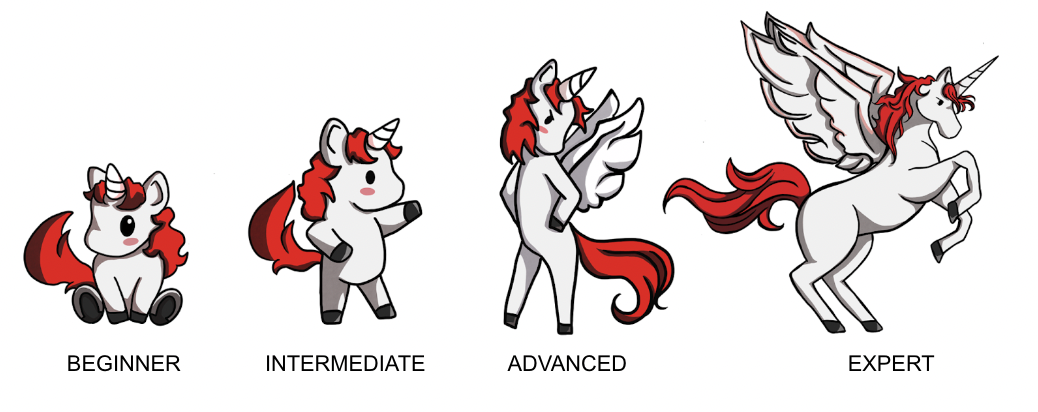
在整個指南中，我們使用 Keras 的官方吉祥物 Keras 教授作為視覺參考，以表示教材的複雜程度

drawing

!pip install -q --upgrade keras-nlp
!pip install -q --upgrade keras  # Upgrade to Keras 3.

import os

os.environ["KERAS_BACKEND"] = "jax"  # or "tensorflow" or "torch"

import keras_nlp
import keras

# Use mixed precision to speed up all training in this guide.
keras.mixed_precision.set_global_policy("mixed_float16")

API 快速入門

我們最高級別的 API 是 keras_nlp.models。這些符號涵蓋了將字串轉換為詞彙、詞彙轉換為密集特徵，以及密集特徵轉換為任務特定輸出的完整使用者旅程。對於每個 XX 架構（例如，Bert），我們提供以下模組

詞彙器：keras_nlp.models.XXTokenizer
- 功能：將字串轉換為詞彙 ID 序列。
- 重要性：字串的原始位元組維度過高，無法用作有用的特徵，因此我們首先將它們映射到少量詞彙，例如將 "The quick brown fox" 映射到 ["the", "qu", "##ick", "br", "##own", "fox"]。
- 繼承自：keras.layers.Layer。
預處理器：keras_nlp.models.XXPreprocessor
- 功能：將字串轉換為由骨幹模型使用的預處理張量字典，從詞彙化開始。
- 重要性：每個模型都使用特殊的詞彙和額外的張量來理解輸入，例如劃分輸入片段和識別填充詞彙。將每個序列填充到相同的長度可以提高計算效率。
- 包含：XXTokenizer。
- 繼承自：keras.layers.Layer。
骨幹模型：keras_nlp.models.XXBackbone
- 功能：將預處理的張量轉換為密集特徵。*不處理字串；請先呼叫預處理器。*
- 重要性：骨幹模型將輸入詞彙提取為可用於下游任務的密集特徵。它通常使用大量的未標記資料在語言建模任務上進行預先訓練。將這些資訊轉移到新任務是現代自然語言處理的一項重大突破。
- 繼承自：keras.Model。
任務：例如，keras_nlp.models.XXClassifier
- 功能：將字串轉換為任務特定的輸出（例如，分類機率）。
- 重要性：任務模型將字串預處理和骨幹模型與任務特定的 Layers 結合起來，以解決句子分類、詞彙分類或文字生成等問題。額外的 Layers 必須使用標記資料進行微調。
- 包含：XXBackbone 和 XXPreprocessor。
- 繼承自：keras.Model。

以下是 BertClassifier 的模組化層次結構（所有關係都是組合的）

drawing

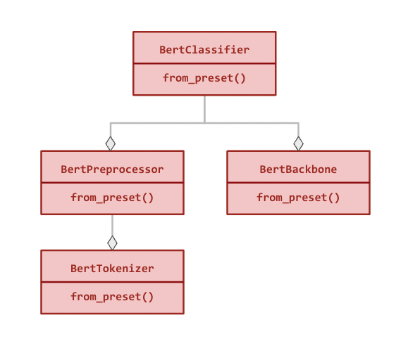
所有模組都可以獨立使用，並且除了使用預設架構和權重實例化類別的標準建構函式之外，還有一個 from_preset() 方法（請參閱以下範例）。

資料

我們將使用 IMDB 電影評論的情緒分析作為範例。在此任務中，我們使用文字來預測評論是正面（label = 1）還是負面（label = 0）。

我們使用 keras.utils.text_dataset_from_directory 載入資料，該方法利用了強大的 tf.data.Dataset 格式來處理範例。

!curl -O https://ai.stanford.edu/~amaas/data/sentiment/aclImdb_v1.tar.gz
!tar -xf aclImdb_v1.tar.gz
!# Remove unsupervised examples
!rm -r aclImdb/train/unsup

BATCH_SIZE = 16
imdb_train = keras.utils.text_dataset_from_directory(
    "aclImdb/train",
    batch_size=BATCH_SIZE,
)
imdb_test = keras.utils.text_dataset_from_directory(
    "aclImdb/test",
    batch_size=BATCH_SIZE,
)

# Inspect first review
# Format is (review text tensor, label tensor)
print(imdb_train.unbatch().take(1).get_single_element())

  % Total    % Received % Xferd  Average Speed   Time    Time     Time  Current
                                 Dload  Upload   Total   Spent    Left  Speed
100 80.2M  100 80.2M    0     0  88.0M      0 --:--:-- --:--:-- --:--:-- 87.9M

Found 25000 files belonging to 2 classes.
Found 25000 files belonging to 2 classes.
(<tf.Tensor: shape=(), dtype=string, numpy=b'This is a very, very early Bugs Bunny cartoon. As a result, the character is still in a transition period--he is not drawn as elongated as he later was and his voice isn\'t quite right. In addition, the chemistry between Elmer and Bugs is a little unusual. Elmer is some poor sap who buys Bugs from a pet shop--there is no gun or desire on his part to blast the bunny to smithereens! However, despite this, this is still a very enjoyable film. The early Bugs was definitely more sassy and cruel than his later incarnations. In later films, he messed with Elmer, Yosimite Sam and others because they started it--they messed with the rabbit. But, in this film, he is much more like Daffy Duck of the late 30s and early 40s--a jerk who just loves irritating others!! A true "anarchist" instead of the hero of the later cartoons. While this isn\'t among the best Bug Bunny cartoons, it sure is fun to watch and it\'s interesting to see just how much he\'s changed over the years.'>, <tf.Tensor: shape=(), dtype=int32, numpy=1>)

使用預先訓練好的分類器進行推論

drawing

KerasNLP 中最高級別的模組是任務。任務是一個 keras.Model，由一個（通常是預先訓練好的）骨幹模型和任務特定的層組成。以下是使用 keras_nlp.models.BertClassifier 的範例。

注意：輸出是每個類別的 logits（例如，[0, 0] 表示正面的機率為 50%）。對於二元分類，輸出為 [負面，正面]。

classifier = keras_nlp.models.BertClassifier.from_preset("bert_tiny_en_uncased_sst2")
# Note: batched inputs expected so must wrap string in iterable
classifier.predict(["I love modular workflows in keras-nlp!"])

 1/1 ━━━━━━━━━━━━━━━━━━━━ 1s 689ms/step

array([[-1.539,  1.543]], dtype=float16)

所有任務都有一個 from_preset 方法，可以用預設的預處理、架構和權重建構一個 keras.Model 實例。這意味著我們可以傳遞任何 keras.Model 接受的格式的原始字串，並獲得特定於我們任務的輸出。

這個特定的預設設定是一個在 sst2 上微調的 "bert_tiny_uncased_en" 骨幹，這是另一個電影評論情感分析（這次來自爛番茄）。我們出於演示目的使用 tiny 架構，但建議使用更大的模型來獲得 SoTA 性能。如需 BertClassifier 可用的所有特定於任務的預設設定，請參閱我們的 keras.io 模型頁面。

讓我們在 IMDB 資料集上評估我們的分類器。您會注意到我們不需要在這裡呼叫 keras.Model.compile。所有任務模型（如 BertClassifier）都附帶編譯預設值，這意味著我們可以直接呼叫 keras.Model.evaluate。您始終可以像往常一樣呼叫編譯來覆蓋這些預設值（例如，添加新指標）。

以下輸出是 [損失，準確度]，

classifier.evaluate(imdb_test)

 1563/1563 ━━━━━━━━━━━━━━━━━━━━ 4s 2ms/step - loss: 0.4610 - sparse_categorical_accuracy: 0.7882

[0.4630218744277954, 0.783519983291626]

我們的結果是在沒有經過任何訓練的情況下準確度達到 78%。還不錯！

微調預先訓練的 BERT 骨幹

drawing

當可以使用特定於我們任務的標記文字時，微調自定義分類器可以提高性能。如果我們想預測 IMDB 評論的情感，使用 IMDB 數據應該比爛番茄數據表現更好！對於許多任務，將沒有可用的相關預先訓練模型（例如，對客戶評論進行分類）。

微調的工作流程與上述幾乎相同，只是我們請求的是僅適用於骨幹模型的預設設定，而不是整個分類器。當傳遞骨幹 預設設定時，任務 Model 將隨機初始化所有特定於任務的層，為訓練做好準備。如需 BertClassifier 可用的所有骨幹預設設定，請參閱我們的 keras.io 模型頁面。

要訓練您的分類器，請像使用任何其他 keras.Model 一樣使用 keras.Model.fit。與我們的推理示例一樣，我們可以依賴任務的編譯預設值並跳過 keras.Model.compile。由於包含預處理，我們再次傳遞原始數據。

classifier = keras_nlp.models.BertClassifier.from_preset(
    "bert_tiny_en_uncased",
    num_classes=2,
)
classifier.fit(
    imdb_train,
    validation_data=imdb_test,
    epochs=1,
)

 1563/1563 ━━━━━━━━━━━━━━━━━━━━ 16s 9ms/step - loss: 0.5202 - sparse_categorical_accuracy: 0.7281 - val_loss: 0.3254 - val_sparse_categorical_accuracy: 0.8621

<keras.src.callbacks.history.History at 0x7f281ffc9f90>

在這裡，我們看到僅經過一個時期的訓練，驗證準確度就顯著提高（0.78 -> 0.87），儘管 IMDB 數據集比 sst2 小得多。

使用使用者控制的預處理進行微調

drawing

對於某些高級訓練場景，用戶可能更喜歡直接控制預處理。對於大型數據集，可以使用 tf.data.experimental.service 預先對示例進行預處理並將其保存到磁碟，或由單獨的工作線程池進行預處理。在其他情況下，需要自定義預處理來處理輸入。

將 preprocessor=None 傳遞給任務 Model 的建構函式以跳過自動預處理，或者傳遞自定義的 BertPreprocessor。

從相同的預設設定中分離預處理

每個模型架構都有一個具有自己的 from_preset 建構函式的並行預處理器 Layer。對此 Layer 使用相同的預設設定將返回與任務匹配的預處理器。

在此工作流程中，我們使用 tf.data.Dataset.cache() 訓練模型三個時期，它在擬合開始之前計算一次預處理並快取結果。

注意：我們可以使用 tf.data 在 Jax 或 PyTorch 後端運行時進行預處理。輸入數據集將在訓練期間自動轉換為後端原生張量類型。事實上，考慮到 tf.data 運行預處理的效率，這在所有後端都是很好的做法。

import tensorflow as tf

preprocessor = keras_nlp.models.BertPreprocessor.from_preset(
    "bert_tiny_en_uncased",
    sequence_length=512,
)

# Apply the preprocessor to every sample of train and test data using `map()`.
# [`tf.data.AUTOTUNE`](https://tensorflow.dev.org.tw/api_docs/python/tf/data/AUTOTUNE) and `prefetch()` are options to tune performance, see
# https://tensorflow.dev.org.tw/guide/data_performance for details.

# Note: only call `cache()` if you training data fits in CPU memory!
imdb_train_cached = (
    imdb_train.map(preprocessor, tf.data.AUTOTUNE).cache().prefetch(tf.data.AUTOTUNE)
)
imdb_test_cached = (
    imdb_test.map(preprocessor, tf.data.AUTOTUNE).cache().prefetch(tf.data.AUTOTUNE)
)

classifier = keras_nlp.models.BertClassifier.from_preset(
    "bert_tiny_en_uncased", preprocessor=None, num_classes=2
)
classifier.fit(
    imdb_train_cached,
    validation_data=imdb_test_cached,
    epochs=3,
)

Epoch 1/3
 1563/1563 ━━━━━━━━━━━━━━━━━━━━ 15s 8ms/step - loss: 0.5194 - sparse_categorical_accuracy: 0.7272 - val_loss: 0.3032 - val_sparse_categorical_accuracy: 0.8728
Epoch 2/3
 1563/1563 ━━━━━━━━━━━━━━━━━━━━ 10s 7ms/step - loss: 0.2871 - sparse_categorical_accuracy: 0.8805 - val_loss: 0.2809 - val_sparse_categorical_accuracy: 0.8818
Epoch 3/3
 1563/1563 ━━━━━━━━━━━━━━━━━━━━ 10s 7ms/step - loss: 0.2134 - sparse_categorical_accuracy: 0.9178 - val_loss: 0.3043 - val_sparse_categorical_accuracy: 0.8790

<keras.src.callbacks.history.History at 0x7f281ffc87f0>

經過三個時期後，我們的驗證準確度僅提高到 0.88。這與我們數據集的小規模和我們的模型都有關係。要超過 90% 的準確度，請嘗試更大的預設模型，例如 "bert_base_en_uncased"。如需 BertClassifier 可用的所有骨幹預設模型，請參閱我們的 keras.io 模型頁面。

自訂預處理

如果需要自訂預處理，我們可以直接訪問將原始字串映射到詞元的 Tokenizer 類別。它還有一個 from_preset() 建構函數，用於取得與預訓練相符的詞彙表。

注意：BertTokenizer 預設不會填充序列，因此輸出是不規則的（每個序列的長度不同）。以下的 MultiSegmentPacker 處理將這些不規則序列填充為密集張量類型（例如 tf.Tensor 或 torch.Tensor）。

tokenizer = keras_nlp.models.BertTokenizer.from_preset("bert_tiny_en_uncased")
tokenizer(["I love modular workflows!", "Libraries over frameworks!"])

# Write your own packer or use one of our `Layers`
packer = keras_nlp.layers.MultiSegmentPacker(
    start_value=tokenizer.cls_token_id,
    end_value=tokenizer.sep_token_id,
    # Note: This cannot be longer than the preset's `sequence_length`, and there
    # is no check for a custom preprocessor!
    sequence_length=64,
)


# This function that takes a text sample `x` and its
# corresponding label `y` as input and converts the
# text into a format suitable for input into a BERT model.
def preprocessor(x, y):
    token_ids, segment_ids = packer(tokenizer(x))
    x = {
        "token_ids": token_ids,
        "segment_ids": segment_ids,
        "padding_mask": token_ids != 0,
    }
    return x, y


imdb_train_preprocessed = imdb_train.map(preprocessor, tf.data.AUTOTUNE).prefetch(
    tf.data.AUTOTUNE
)
imdb_test_preprocessed = imdb_test.map(preprocessor, tf.data.AUTOTUNE).prefetch(
    tf.data.AUTOTUNE
)

# Preprocessed example
print(imdb_train_preprocessed.unbatch().take(1).get_single_element())

({'token_ids': <tf.Tensor: shape=(64,), dtype=int32, numpy=
array([  101,  2023,  2003,  2941,  2028,  1997,  2026,  5440,  3152,
        1010,  1045,  2052, 16755,  2008,  3071, 12197,  2009,  1012,
        2045,  2003,  2070,  2307,  3772,  1999,  2009,  1998,  2009,
        3065,  2008,  2025,  2035,  1000,  2204,  1000,  3152,  2024,
        2137,  1012,  1012,  1012,  1012,   102,     0,     0,     0,
           0,     0,     0,     0,     0,     0,     0,     0,     0,
           0,     0,     0,     0,     0,     0,     0,     0,     0,
           0], dtype=int32)>, 'segment_ids': <tf.Tensor: shape=(64,), dtype=int32, numpy=
array([0, 0, 0, 0, 0, 0, 0, 0, 0, 0, 0, 0, 0, 0, 0, 0, 0, 0, 0, 0, 0, 0,
       0, 0, 0, 0, 0, 0, 0, 0, 0, 0, 0, 0, 0, 0, 0, 0, 0, 0, 0, 0, 0, 0,
       0, 0, 0, 0, 0, 0, 0, 0, 0, 0, 0, 0, 0, 0, 0, 0, 0, 0, 0, 0],
      dtype=int32)>, 'padding_mask': <tf.Tensor: shape=(64,), dtype=bool, numpy=
array([ True,  True,  True,  True,  True,  True,  True,  True,  True,
        True,  True,  True,  True,  True,  True,  True,  True,  True,
        True,  True,  True,  True,  True,  True,  True,  True,  True,
        True,  True,  True,  True,  True,  True,  True,  True,  True,
        True,  True,  True,  True,  True,  True, False, False, False,
       False, False, False, False, False, False, False, False, False,
       False, False, False, False, False, False, False, False, False,
       False])>}, <tf.Tensor: shape=(), dtype=int32, numpy=1>)

使用自訂模型進行微調

drawing

對於更進階的應用程式，可能沒有適當的任務 Model 可用。在這種情況下，我們可以直接訪問骨幹 Model，它有自己的 from_preset 建構函數，並且可以與自訂 Layer 組合。詳細範例請參閱我們的遷移學習指南。

骨幹 Model 不包含自動預處理，但可以使用與先前工作流程中顯示的相同預設模型與匹配的預處理器配對。

在此工作流程中，我們嘗試凍結骨幹模型並添加兩個可訓練的 Transformer 層以適應新的輸入。

注意：我們可以忽略有關 pooled_dense 層梯度的警告，因為我們使用的是 BERT 的序列輸出。

preprocessor = keras_nlp.models.BertPreprocessor.from_preset("bert_tiny_en_uncased")
backbone = keras_nlp.models.BertBackbone.from_preset("bert_tiny_en_uncased")

imdb_train_preprocessed = (
    imdb_train.map(preprocessor, tf.data.AUTOTUNE).cache().prefetch(tf.data.AUTOTUNE)
)
imdb_test_preprocessed = (
    imdb_test.map(preprocessor, tf.data.AUTOTUNE).cache().prefetch(tf.data.AUTOTUNE)
)

backbone.trainable = False
inputs = backbone.input
sequence = backbone(inputs)["sequence_output"]
for _ in range(2):
    sequence = keras_nlp.layers.TransformerEncoder(
        num_heads=2,
        intermediate_dim=512,
        dropout=0.1,
    )(sequence)
# Use [CLS] token output to classify
outputs = keras.layers.Dense(2)(sequence[:, backbone.cls_token_index, :])

model = keras.Model(inputs, outputs)
model.compile(
    loss=keras.losses.SparseCategoricalCrossentropy(from_logits=True),
    optimizer=keras.optimizers.AdamW(5e-5),
    metrics=[keras.metrics.SparseCategoricalAccuracy()],
    jit_compile=True,
)
model.summary()
model.fit(
    imdb_train_preprocessed,
    validation_data=imdb_test_preprocessed,
    epochs=3,
)

Model: "functional_1"

┏━━━━━━━━━━━━━━━━━━━━━┳━━━━━━━━━━━━━━━━━━━┳━━━━━━━━━┳━━━━━━━━━━━━━━━━━━━━━━┓
┃ Layer (type)        ┃ Output Shape      ┃ Param # ┃ Connected to         ┃
┡━━━━━━━━━━━━━━━━━━━━━╇━━━━━━━━━━━━━━━━━━━╇━━━━━━━━━╇━━━━━━━━━━━━━━━━━━━━━━┩
│ padding_mask        │ (None, None)      │       0 │ -                    │
│ (InputLayer)        │                   │         │                      │
├─────────────────────┼───────────────────┼─────────┼──────────────────────┤
│ segment_ids         │ (None, None)      │       0 │ -                    │
│ (InputLayer)        │                   │         │                      │
├─────────────────────┼───────────────────┼─────────┼──────────────────────┤
│ token_ids           │ (None, None)      │       0 │ -                    │
│ (InputLayer)        │                   │         │                      │
├─────────────────────┼───────────────────┼─────────┼──────────────────────┤
│ bert_backbone_3     │ [(None, 128),     │ 4,385,… │ padding_mask[0][0],  │
│ (BertBackbone)      │ (None, None,      │         │ segment_ids[0][0],   │
│                     │ 128)]             │         │ token_ids[0][0]      │
├─────────────────────┼───────────────────┼─────────┼──────────────────────┤
│ transformer_encoder │ (None, None, 128) │ 198,272 │ bert_backbone_3[0][… │
│ (TransformerEncode… │                   │         │                      │
├─────────────────────┼───────────────────┼─────────┼──────────────────────┤
│ transformer_encode… │ (None, None, 128) │ 198,272 │ transformer_encoder… │
│ (TransformerEncode… │                   │         │                      │
├─────────────────────┼───────────────────┼─────────┼──────────────────────┤
│ get_item_4          │ (None, 128)       │       0 │ transformer_encoder… │
│ (GetItem)           │                   │         │                      │
├─────────────────────┼───────────────────┼─────────┼──────────────────────┤
│ dense (Dense)       │ (None, 2)         │     258 │ get_item_4[0][0]     │
└─────────────────────┴───────────────────┴─────────┴──────────────────────┘

 Total params: 4,782,722 (18.24 MB)

 Trainable params: 396,802 (1.51 MB)

 Non-trainable params: 4,385,920 (16.73 MB)

Epoch 1/3
 1563/1563 ━━━━━━━━━━━━━━━━━━━━ 17s 10ms/step - loss: 0.6208 - sparse_categorical_accuracy: 0.6612 - val_loss: 0.6119 - val_sparse_categorical_accuracy: 0.6758
Epoch 2/3
 1563/1563 ━━━━━━━━━━━━━━━━━━━━ 12s 8ms/step - loss: 0.5324 - sparse_categorical_accuracy: 0.7347 - val_loss: 0.5484 - val_sparse_categorical_accuracy: 0.7320
Epoch 3/3
 1563/1563 ━━━━━━━━━━━━━━━━━━━━ 12s 8ms/step - loss: 0.4735 - sparse_categorical_accuracy: 0.7723 - val_loss: 0.4874 - val_sparse_categorical_accuracy: 0.7742

<keras.src.callbacks.history.History at 0x7f2790170220>

儘管可訓練參數只有 BertClassifier 模型的 10%，但此模型仍可達到合理的準確度。每個訓練步驟大約需要 1/3 的時間，即使考慮到快取的預處理也是如此。

預先訓練骨幹模型

drawing

您是否有權訪問您領域中的大型未標記數據集？它們的大小是否與用於訓練熱門骨幹模型（如 BERT、RoBERTa 或 GPT2）的大小（XX+ GiB）相同？如果是這樣，您可能會從您自己領域特定骨幹模型的預訓練中受益。

自然語言處理模型通常在語言建模任務上進行預訓練，根據輸入句子中的可見詞預測被遮蔽的詞。例如，給定輸入 "The fox [MASK] over the [MASK] dog"，模型可能會被要求預測 ["jumped", "lazy"]。然後，此模型的較低層將打包為骨幹，並與與新任務相關的層組合。

KerasNLP 函式庫提供了 SoTA 骨幹和詞元化器，可以在沒有預設模型的情況下從頭開始訓練。

在此工作流程中，我們使用 IMDB 評論文字預訓練 BERT 骨幹。我們跳過了「下一句預測」(NSP) 損失，因為它顯著增加了數據處理的複雜性，並且在後來的模型（如 RoBERTa）中被捨棄。請參閱我們的端到端 Transformer 預訓練，以獲取有關如何複製原始論文的逐步詳細資訊。

預處理

# All BERT `en` models have the same vocabulary, so reuse preprocessor from
# "bert_tiny_en_uncased"
preprocessor = keras_nlp.models.BertPreprocessor.from_preset(
    "bert_tiny_en_uncased",
    sequence_length=256,
)
packer = preprocessor.packer
tokenizer = preprocessor.tokenizer

# keras.Layer to replace some input tokens with the "[MASK]" token
masker = keras_nlp.layers.MaskedLMMaskGenerator(
    vocabulary_size=tokenizer.vocabulary_size(),
    mask_selection_rate=0.25,
    mask_selection_length=64,
    mask_token_id=tokenizer.token_to_id("[MASK]"),
    unselectable_token_ids=[
        tokenizer.token_to_id(x) for x in ["[CLS]", "[PAD]", "[SEP]"]
    ],
)


def preprocess(inputs, label):
    inputs = preprocessor(inputs)
    masked_inputs = masker(inputs["token_ids"])
    # Split the masking layer outputs into a (features, labels, and weights)
    # tuple that we can use with keras.Model.fit().
    features = {
        "token_ids": masked_inputs["token_ids"],
        "segment_ids": inputs["segment_ids"],
        "padding_mask": inputs["padding_mask"],
        "mask_positions": masked_inputs["mask_positions"],
    }
    labels = masked_inputs["mask_ids"]
    weights = masked_inputs["mask_weights"]
    return features, labels, weights


pretrain_ds = imdb_train.map(preprocess, num_parallel_calls=tf.data.AUTOTUNE).prefetch(
    tf.data.AUTOTUNE
)
pretrain_val_ds = imdb_test.map(
    preprocess, num_parallel_calls=tf.data.AUTOTUNE
).prefetch(tf.data.AUTOTUNE)

# Tokens with ID 103 are "masked"
print(pretrain_ds.unbatch().take(1).get_single_element())

({'token_ids': <tf.Tensor: shape=(256,), dtype=int32, numpy=
array([  101,   103,  2332,   103,  1006,   103,   103,  2332,  2370,
        1007,   103,  2029,   103,  2402,  2155,  1010, 24159,  2000,
        3541,  7081,  1010,  2424,  2041,  2055,  1996,  9004,  4528,
         103,   103,  2037,  2188,   103,  1996,  2269,  1006,  8512,
        3054,   103,  4246,  1007,  2059,  4858,  1555,  2055,  1996,
       23025, 22911,  8940,  2598,  3458,  1996, 25483,  4528,  2008,
        2038,   103,  1997, 15218,  1011,   103,  1997,   103,  2505,
        3950,  2045,  3310,  2067,  2025,  3243,  2157,  1012,   103,
        7987,  1013,  1028,   103,  7987,  1013,  1028,  2917,   103,
        1000,  5469,  1000,   103,   103,  2041, 22902,  1010, 23979,
        1010,  1998,  1999, 23606,   103,  1998,  4247,  2008,  2126,
        2005,  1037,  2096,  1010,  2007,  1996,   103,  5409,   103,
        2108,  3054,  3211,  4246,  1005,  1055, 22692,  2836,  1012,
        2009,   103,  1037,  2210,  2488,   103,   103,  2203,  1010,
        2007,   103,   103,  9599,  1012,   103,  2391,  1997,  2755,
        1010,  1996,  2878,  3185,  2003,  2428,   103,  1010,   103,
         103,   103,  1045,  2064,  1005,  1056,  3294, 19776,  2009,
        1011,  2012,  2560,  2009,  2038,  2242,  2000,   103,  2009,
       13432,  1012, 11519,  4637,  4616,  2011,  5965,  1043, 11761,
         103,   103,  2004,   103,  7968,  3243,  4793, 11429,  1010,
        1998,  8226,  2665, 18331,  1010,  1219,  1996,  4487, 22747,
        8004, 12165,  4382,  5125,   103,  3597,   103,  2024,  2025,
        2438,  2000,   103,  2417, 21564,  2143,   103,   103,  7987,
        1013,  1028,  1026,   103,  1013,  1028,  2332,  2038,   103,
        5156, 12081,  2004,  1996,   103,  1012,  1026, 14216,   103,
         103,  1026,  7987,  1013,  1028,   184,  2011,  1037,  8297,
        2036,   103,  2011,  2984,   103,  1006,  2003,  2009,  2151,
        4687,  2008,  2016,  1005,  1055,  2018,  2053,  7731,   103,
         103,  2144,  1029,   102], dtype=int32)>, 'segment_ids': <tf.Tensor: shape=(256,), dtype=int32, numpy=
array([0, 0, 0, 0, 0, 0, 0, 0, 0, 0, 0, 0, 0, 0, 0, 0, 0, 0, 0, 0, 0, 0,
       0, 0, 0, 0, 0, 0, 0, 0, 0, 0, 0, 0, 0, 0, 0, 0, 0, 0, 0, 0, 0, 0,
       0, 0, 0, 0, 0, 0, 0, 0, 0, 0, 0, 0, 0, 0, 0, 0, 0, 0, 0, 0, 0, 0,
       0, 0, 0, 0, 0, 0, 0, 0, 0, 0, 0, 0, 0, 0, 0, 0, 0, 0, 0, 0, 0, 0,
       0, 0, 0, 0, 0, 0, 0, 0, 0, 0, 0, 0, 0, 0, 0, 0, 0, 0, 0, 0, 0, 0,
       0, 0, 0, 0, 0, 0, 0, 0, 0, 0, 0, 0, 0, 0, 0, 0, 0, 0, 0, 0, 0, 0,
       0, 0, 0, 0, 0, 0, 0, 0, 0, 0, 0, 0, 0, 0, 0, 0, 0, 0, 0, 0, 0, 0,
       0, 0, 0, 0, 0, 0, 0, 0, 0, 0, 0, 0, 0, 0, 0, 0, 0, 0, 0, 0, 0, 0,
       0, 0, 0, 0, 0, 0, 0, 0, 0, 0, 0, 0, 0, 0, 0, 0, 0, 0, 0, 0, 0, 0,
       0, 0, 0, 0, 0, 0, 0, 0, 0, 0, 0, 0, 0, 0, 0, 0, 0, 0, 0, 0, 0, 0,
       0, 0, 0, 0, 0, 0, 0, 0, 0, 0, 0, 0, 0, 0, 0, 0, 0, 0, 0, 0, 0, 0,
       0, 0, 0, 0, 0, 0, 0, 0, 0, 0, 0, 0, 0, 0], dtype=int32)>, 'padding_mask': <tf.Tensor: shape=(256,), dtype=bool, numpy=
array([ True,  True,  True,  True,  True,  True,  True,  True,  True,
        True,  True,  True,  True,  True,  True,  True,  True,  True,
        True,  True,  True,  True,  True,  True,  True,  True,  True,
        True,  True,  True,  True,  True,  True,  True,  True,  True,
        True,  True,  True,  True,  True,  True,  True,  True,  True,
        True,  True,  True,  True,  True,  True,  True,  True,  True,
        True,  True,  True,  True,  True,  True,  True,  True,  True,
        True,  True,  True,  True,  True,  True,  True,  True,  True,
        True,  True,  True,  True,  True,  True,  True,  True,  True,
        True,  True,  True,  True,  True,  True,  True,  True,  True,
        True,  True,  True,  True,  True,  True,  True,  True,  True,
        True,  True,  True,  True,  True,  True,  True,  True,  True,
        True,  True,  True,  True,  True,  True,  True,  True,  True,
        True,  True,  True,  True,  True,  True,  True,  True,  True,
        True,  True,  True,  True,  True,  True,  True,  True,  True,
        True,  True,  True,  True,  True,  True,  True,  True,  True,
        True,  True,  True,  True,  True,  True,  True,  True,  True,
        True,  True,  True,  True,  True,  True,  True,  True,  True,
        True,  True,  True,  True,  True,  True,  True,  True,  True,
        True,  True,  True,  True,  True,  True,  True,  True,  True,
        True,  True,  True,  True,  True,  True,  True,  True,  True,
        True,  True,  True,  True,  True,  True,  True,  True,  True,
        True,  True,  True,  True,  True,  True,  True,  True,  True,
        True,  True,  True,  True,  True,  True,  True,  True,  True,
        True,  True,  True,  True,  True,  True,  True,  True,  True,
        True,  True,  True,  True,  True,  True,  True,  True,  True,
        True,  True,  True,  True,  True,  True,  True,  True,  True,
        True,  True,  True,  True,  True,  True,  True,  True,  True,
        True,  True,  True,  True])>, 'mask_positions': <tf.Tensor: shape=(64,), dtype=int64, numpy=
array([  1,   3,   5,   6,  10,  12,  13,  27,  28,  31,  37,  42,  51,
        55,  59,  61,  65,  71,  75,  80,  83,  84,  85,  94, 105, 107,
       108, 118, 122, 123, 127, 128, 131, 141, 143, 144, 145, 149, 160,
       167, 170, 171, 172, 174, 176, 185, 193, 195, 200, 204, 205, 208,
       210, 215, 220, 223, 224, 225, 230, 231, 235, 238, 251, 252])>}, <tf.Tensor: shape=(64,), dtype=int32, numpy=
array([ 4459,  6789, 22892,  2011,  1999,  1037,  2402,  2485,  2000,
        1012,  3211,  2041,  9004,  4204,  2069,  2607,  3310,  1026,
        1026,  2779,  1000,  3861,  4627,  1010,  7619,  5783,  2108,
        4152,  2646,  1996, 15958, 14888,  1999, 14888,  2029,  2003,
        2339,  1056,  2191,  2011, 11761,  2638,  1010,  1996,  2214,
        2004, 14674,  2860,  2428,  1012,  1026,  1028,  7987,  2010,
        2704,  7987,  1013,  1028,  2628,  2011,  2856, 12838,  2143,
        2147], dtype=int32)>, <tf.Tensor: shape=(64,), dtype=float16, numpy=
array([1., 1., 1., 1., 1., 1., 1., 1., 1., 1., 1., 1., 1., 1., 1., 1., 1.,
       1., 1., 1., 1., 1., 1., 1., 1., 1., 1., 1., 1., 1., 1., 1., 1., 1.,
       1., 1., 1., 1., 1., 1., 1., 1., 1., 1., 1., 1., 1., 1., 1., 1., 1.,
       1., 1., 1., 1., 1., 1., 1., 1., 1., 1., 1., 1., 1.], dtype=float16)>)

預訓練模型

# BERT backbone
backbone = keras_nlp.models.BertBackbone(
    vocabulary_size=tokenizer.vocabulary_size(),
    num_layers=2,
    num_heads=2,
    hidden_dim=128,
    intermediate_dim=512,
)

# Language modeling head
mlm_head = keras_nlp.layers.MaskedLMHead(
    token_embedding=backbone.token_embedding,
)

inputs = {
    "token_ids": keras.Input(shape=(None,), dtype=tf.int32, name="token_ids"),
    "segment_ids": keras.Input(shape=(None,), dtype=tf.int32, name="segment_ids"),
    "padding_mask": keras.Input(shape=(None,), dtype=tf.int32, name="padding_mask"),
    "mask_positions": keras.Input(shape=(None,), dtype=tf.int32, name="mask_positions"),
}

# Encoded token sequence
sequence = backbone(inputs)["sequence_output"]

# Predict an output word for each masked input token.
# We use the input token embedding to project from our encoded vectors to
# vocabulary logits, which has been shown to improve training efficiency.
outputs = mlm_head(sequence, mask_positions=inputs["mask_positions"])

# Define and compile our pretraining model.
pretraining_model = keras.Model(inputs, outputs)
pretraining_model.summary()
pretraining_model.compile(
    loss=keras.losses.SparseCategoricalCrossentropy(from_logits=True),
    optimizer=keras.optimizers.AdamW(learning_rate=5e-4),
    weighted_metrics=[keras.metrics.SparseCategoricalAccuracy()],
    jit_compile=True,
)

# Pretrain on IMDB dataset
pretraining_model.fit(
    pretrain_ds,
    validation_data=pretrain_val_ds,
    epochs=3,  # Increase to 6 for higher accuracy
)

Model: "functional_3"

┏━━━━━━━━━━━━━━━━━━━━━┳━━━━━━━━━━━━━━━━━━━┳━━━━━━━━━┳━━━━━━━━━━━━━━━━━━━━━━┓
┃ Layer (type)        ┃ Output Shape      ┃ Param # ┃ Connected to         ┃
┡━━━━━━━━━━━━━━━━━━━━━╇━━━━━━━━━━━━━━━━━━━╇━━━━━━━━━╇━━━━━━━━━━━━━━━━━━━━━━┩
│ mask_positions      │ (None, None)      │       0 │ -                    │
│ (InputLayer)        │                   │         │                      │
├─────────────────────┼───────────────────┼─────────┼──────────────────────┤
│ padding_mask        │ (None, None)      │       0 │ -                    │
│ (InputLayer)        │                   │         │                      │
├─────────────────────┼───────────────────┼─────────┼──────────────────────┤
│ segment_ids         │ (None, None)      │       0 │ -                    │
│ (InputLayer)        │                   │         │                      │
├─────────────────────┼───────────────────┼─────────┼──────────────────────┤
│ token_ids           │ (None, None)      │       0 │ -                    │
│ (InputLayer)        │                   │         │                      │
├─────────────────────┼───────────────────┼─────────┼──────────────────────┤
│ bert_backbone_4     │ [(None, 128),     │ 4,385,… │ mask_positions[0][0… │
│ (BertBackbone)      │ (None, None,      │         │ padding_mask[0][0],  │
│                     │ 128)]             │         │ segment_ids[0][0],   │
│                     │                   │         │ token_ids[0][0]      │
├─────────────────────┼───────────────────┼─────────┼──────────────────────┤
│ masked_lm_head      │ (None, None,      │ 3,954,… │ bert_backbone_4[0][… │
│ (MaskedLMHead)      │ 30522)            │         │ mask_positions[0][0] │
└─────────────────────┴───────────────────┴─────────┴──────────────────────┘

 Total params: 4,433,210 (16.91 MB)

 Trainable params: 4,433,210 (16.91 MB)

 Non-trainable params: 0 (0.00 B)

Epoch 1/3
 1563/1563 ━━━━━━━━━━━━━━━━━━━━ 22s 12ms/step - loss: 5.7032 - sparse_categorical_accuracy: 0.0566 - val_loss: 5.0685 - val_sparse_categorical_accuracy: 0.1044
Epoch 2/3
 1563/1563 ━━━━━━━━━━━━━━━━━━━━ 13s 8ms/step - loss: 5.0701 - sparse_categorical_accuracy: 0.1096 - val_loss: 4.9363 - val_sparse_categorical_accuracy: 0.1239
Epoch 3/3
 1563/1563 ━━━━━━━━━━━━━━━━━━━━ 13s 8ms/step - loss: 4.9607 - sparse_categorical_accuracy: 0.1240 - val_loss: 4.7913 - val_sparse_categorical_accuracy: 0.1417

<keras.src.callbacks.history.History at 0x7f2738299330>

預訓練後，請儲存您的 backbone 子模型以在新任務中使用！

從頭開始建構和訓練您自己的 Transformer 模型

drawing

想實作一種新穎的 Transformer 架構嗎？KerasNLP 函式庫在我們的 models API 中提供了所有用於建構 SoTA 架構的低階模組。這包括 keras_nlp.tokenizers API，它允許您使用 WordPieceTokenizer、BytePairTokenizer 或 SentencePieceTokenizer 訓練您自己的子詞分詞器。

在此工作流程中，我們在 IMDB 資料上訓練了一個自訂分詞器，並設計了一個具有自訂 Transformer 架構的骨幹網路。為簡單起見，我們接著直接針對分類任務進行訓練。想了解更多細節嗎？我們在 keras.io 上撰寫了一份關於預先訓練和微調自訂 Transformer 的完整指南。

從 IMDB 資料訓練自訂詞彙

vocab = keras_nlp.tokenizers.compute_word_piece_vocabulary(
    imdb_train.map(lambda x, y: x),
    vocabulary_size=20_000,
    lowercase=True,
    strip_accents=True,
    reserved_tokens=["[PAD]", "[START]", "[END]", "[MASK]", "[UNK]"],
)
tokenizer = keras_nlp.tokenizers.WordPieceTokenizer(
    vocabulary=vocab,
    lowercase=True,
    strip_accents=True,
    oov_token="[UNK]",
)

使用自訂分詞器預先處理資料

packer = keras_nlp.layers.StartEndPacker(
    start_value=tokenizer.token_to_id("[START]"),
    end_value=tokenizer.token_to_id("[END]"),
    pad_value=tokenizer.token_to_id("[PAD]"),
    sequence_length=512,
)


def preprocess(x, y):
    token_ids = packer(tokenizer(x))
    return token_ids, y


imdb_preproc_train_ds = imdb_train.map(
    preprocess, num_parallel_calls=tf.data.AUTOTUNE
).prefetch(tf.data.AUTOTUNE)
imdb_preproc_val_ds = imdb_test.map(
    preprocess, num_parallel_calls=tf.data.AUTOTUNE
).prefetch(tf.data.AUTOTUNE)

print(imdb_preproc_train_ds.unbatch().take(1).get_single_element())

(<tf.Tensor: shape=(512,), dtype=int32, numpy=
array([    1,   102,    11,    61,    43,   771,    16,   340,   916,
        1259,   155,    16,   135,   207,    18,   501, 10568,   344,
          16,    51,   206,   612,   211,   232,    43,  1094,    17,
         215,   155,   103,   238,   202,    18,   111,    16,    51,
         143,  1583,   131,   100,    18,    32,   101,    19,    34,
          32,   101,    19,    34,   102,    11,    61,    43,   155,
         105,  5337,    99,   120,     6,  1289,     6,   129,    96,
         526,    18,   111,    16,   193,    51,   197,   102,    16,
          51,   252,    11,    62,   167,   104,   642,    98,     6,
        8572,     6,   154,    51,   153,  1464,   119,  3005,   990,
        2393,    18,   102,    11,    61,   233,   404,   103,   104,
         110,    18,    18,    18,   233,  1259,    18,    18,    18,
         154,    51,   659, 16273,   867,   192,  1632,   133,   990,
        2393,    18,    32,   101,    19,    34,    32,   101,    19,
          34,    96,   110,  2886,   761,   114,  4905,   293, 12337,
          97,  2375,    18,   113,   143,   158,   179,   104,  4905,
         610,    16, 12585,    97,   516,   725,    18,   113,   323,
          96,   651,   146,   104,   207, 17649,    16,    96,   176,
       16022,   136,    16,  1414,   136,    18,   113,   323,    96,
        2184,    18,    97,   150,   651,    51,   242,   104,   100,
       11722,    18,   113,   151,   543,   102,   171,   115,  1081,
         103,    96,   222,    18,    18,    18,    18,   102,   659,
        1081,    18,    18,    18,   102,    11,    61,   115,   299,
          18,   113,   323,    96,  1579,    98,   203,  4438,  2033,
         103,    96,   222,    18,    18,    18,    32,   101,    19,
          34,    32,   101,    19,    34,   111,    16,    51,   455,
         174,    99,   859,    43,  1687,  3330,    99,   104,  1021,
          18,    18,    18,    51,   181,    11,    62,   214,   138,
          96,   155,   100,   115,   916,    14,  1286,    14,    99,
         296,    96,   642,   105,   224,  4598,   117,  1289,   156,
         103,   904,    16,   111,   115,   103,  1628,    18,   113,
         181,    11,    62,   119,    96,  1054,   155,    16,   111,
         156, 14665,    18,   146,   110,   139,   742,    16,    96,
        4905,   293, 12337,    97,  7042,  1104,   106,   557,   103,
         366,    18,   128,    16,   150,  2446,   135,    96,   960,
          98,    96,  4905,    18,   113,   323,   156,    43,  1174,
         293,   188,    18,    18,    18,    43,   639,   293,    96,
         455,   108,   207,    97,  1893,    99,  1081,   104,  4905,
          18,    51,   194,   104,   440,    98, 12337,    99,  7042,
        1104,   654,   122,    30,     6,    51,   276,    99,   663,
          18,    18,    18,    97,   138,   113,   207,   163,    16,
         113,   171,   172,   107,    51,  1027,   113,     6,    18,
          32,   101,    19,    34,    32,   101,    19,    34,   104,
         110,   171,   333, 10311,   141,  1311,   135,   140,   100,
         207,    97,   140,   100,    99,   120,  1632,    18,    18,
          18,    97,   210,    11,    61,    96,  6236,   293,   188,
          18,    51,   181,    11,    62,   214,   138,    96,   421,
          98,   104,   110,   100,     6,   207, 14129,   122,    18,
          18,    18,   151,  1128,    97,  1632,  1675,     6,   133,
           6,   207,   100,   404,    18,    18,    18,   150,   646,
         179,   133,   210,     6,    18,   111,   103,   152,   744,
          16,   104,   110,   100,   557,    43,  1120,   108,    96,
         701,   382,   105,   102,   260,   113,   194,    18,    18,
          18,     2,     0,     0,     0,     0,     0,     0,     0,
           0,     0,     0,     0,     0,     0,     0,     0,     0,
           0,     0,     0,     0,     0,     0,     0,     0,     0,
           0,     0,     0,     0,     0,     0,     0,     0],
      dtype=int32)>, <tf.Tensor: shape=(), dtype=int32, numpy=1>)

設計一個微型 Transformer

token_id_input = keras.Input(
    shape=(None,),
    dtype="int32",
    name="token_ids",
)
outputs = keras_nlp.layers.TokenAndPositionEmbedding(
    vocabulary_size=len(vocab),
    sequence_length=packer.sequence_length,
    embedding_dim=64,
)(token_id_input)
outputs = keras_nlp.layers.TransformerEncoder(
    num_heads=2,
    intermediate_dim=128,
    dropout=0.1,
)(outputs)
# Use "[START]" token to classify
outputs = keras.layers.Dense(2)(outputs[:, 0, :])
model = keras.Model(
    inputs=token_id_input,
    outputs=outputs,
)

model.summary()

Model: "functional_5"

┏━━━━━━━━━━━━━━━━━━━━━━━━━━━━━━━━━┳━━━━━━━━━━━━━━━━━━━━━━━━━━━┳━━━━━━━━━━━━┓
┃ Layer (type)                    ┃ Output Shape              ┃    Param # ┃
┡━━━━━━━━━━━━━━━━━━━━━━━━━━━━━━━━━╇━━━━━━━━━━━━━━━━━━━━━━━━━━━╇━━━━━━━━━━━━┩
│ token_ids (InputLayer)          │ (None, None)              │          0 │
├─────────────────────────────────┼───────────────────────────┼────────────┤
│ token_and_position_embedding    │ (None, None, 64)          │  1,259,648 │
│ (TokenAndPositionEmbedding)     │                           │            │
├─────────────────────────────────┼───────────────────────────┼────────────┤
│ transformer_encoder_2           │ (None, None, 64)          │     33,472 │
│ (TransformerEncoder)            │                           │            │
├─────────────────────────────────┼───────────────────────────┼────────────┤
│ get_item_6 (GetItem)            │ (None, 64)                │          0 │
├─────────────────────────────────┼───────────────────────────┼────────────┤
│ dense_1 (Dense)                 │ (None, 2)                 │        130 │
└─────────────────────────────────┴───────────────────────────┴────────────┘

 Total params: 1,293,250 (4.93 MB)

 Trainable params: 1,293,250 (4.93 MB)

 Non-trainable params: 0 (0.00 B)

直接針對分類目標訓練 Transformer

model.compile(
    loss=keras.losses.SparseCategoricalCrossentropy(from_logits=True),
    optimizer=keras.optimizers.AdamW(5e-5),
    metrics=[keras.metrics.SparseCategoricalAccuracy()],
    jit_compile=True,
)
model.fit(
    imdb_preproc_train_ds,
    validation_data=imdb_preproc_val_ds,
    epochs=3,
)

Epoch 1/3
 1563/1563 ━━━━━━━━━━━━━━━━━━━━ 8s 4ms/step - loss: 0.7790 - sparse_categorical_accuracy: 0.5367 - val_loss: 0.4420 - val_sparse_categorical_accuracy: 0.8120
Epoch 2/3
 1563/1563 ━━━━━━━━━━━━━━━━━━━━ 5s 3ms/step - loss: 0.3654 - sparse_categorical_accuracy: 0.8443 - val_loss: 0.3046 - val_sparse_categorical_accuracy: 0.8752
Epoch 3/3
 1563/1563 ━━━━━━━━━━━━━━━━━━━━ 5s 3ms/step - loss: 0.2471 - sparse_categorical_accuracy: 0.9019 - val_loss: 0.3060 - val_sparse_categorical_accuracy: 0.8748

<keras.src.callbacks.history.History at 0x7f26d032a4d0>

令人興奮的是，我們自訂分類器的效能與微調 "bert_tiny_en_uncased" 的效能相似！為了看到預先訓練的優勢並超過 90% 的準確率，我們需要使用更大的**預設模型**，例如 "bert_base_en_uncased"。

KerasNLP 入門

◆ 簡介

◆ 資料

從相同的預設設定中分離預處理

自訂預處理

◆ 使用自訂模型進行微調

◆ 預先訓練骨幹網路模型

預處理

預訓練模型

◆ 從頭開始建構和訓練您自己的 Transformer

從 IMDB 資料訓練自訂詞彙

使用自訂分詞器預先處理資料

設計一個微型 Transformer

直接針對分類目標訓練 Transformer