使用內建方法進行訓練與評估
作者: fchollet
建立日期 2019/03/01
上次修改日期 2023/06/25
說明: 使用 fit() 和 evaluate() 進行訓練與評估的完整指南。

設定
# We import torch & TF so as to use torch Dataloaders & tf.data.Datasets.
import torch
import tensorflow as tf

import os
import numpy as np
import keras
from keras import layers
from keras import ops
簡介
本指南涵蓋在使用內建 API 進行訓練與驗證時的模型訓練、評估和預測(推論),例如 Model.fit()、Model.evaluate() 和 Model.predict()。
如果您有興趣在指定自己的訓練步驟函數時利用 fit(),請參閱關於自訂 fit() 中發生的情況的指南
如果您有興趣從頭開始撰寫自己的訓練與評估迴圈,請參閱關於撰寫訓練迴圈的指南
一般來說,無論您是使用內建迴圈還是撰寫自己的迴圈,模型訓練與評估在每一種 Keras 模型(循序模型、使用函數式 API 建立的模型,以及透過模型子類別化從頭開始撰寫的模型)中的運作方式都完全相同。
API 概述:第一個端對端範例
當將資料傳遞至模型的內建訓練迴圈時,您應該使用以下其中一種方式:
- NumPy 陣列(如果您的資料很小且適合放入記憶體)
keras.utils.PyDataset的子類別tf.data.Dataset物件- PyTorch
DataLoader實例
在接下來的幾個段落中,我們將使用 MNIST 資料集作為 NumPy 陣列,以示範如何使用最佳化器、損失和指標。之後,我們將仔細檢視其他每個選項。
讓我們考慮以下模型(這裡我們使用函數式 API 建立,但它也可以是循序模型或子類別化的模型)
inputs = keras.Input(shape=(784,), name="digits")
x = layers.Dense(64, activation="relu", name="dense_1")(inputs)
x = layers.Dense(64, activation="relu", name="dense_2")(x)
outputs = layers.Dense(10, activation="softmax", name="predictions")(x)

model = keras.Model(inputs=inputs, outputs=outputs)
以下是一般端對端工作流程的樣子,包括
- 訓練
- 在從原始訓練資料產生的保留集上進行驗證
- 在測試資料上進行評估
我們將在此範例中使用 MNIST 資料。
(x_train, y_train), (x_test, y_test) = keras.datasets.mnist.load_data()

# Preprocess the data (these are NumPy arrays)
x_train = x_train.reshape(60000, 784).astype("float32") / 255
x_test = x_test.reshape(10000, 784).astype("float32") / 255

y_train = y_train.astype("float32")
y_test = y_test.astype("float32")

# Reserve 10,000 samples for validation
x_val = x_train[-10000:]
y_val = y_train[-10000:]
x_train = x_train[:-10000]
y_train = y_train[:-10000]
我們指定訓練組態(最佳化器、損失、指標)
model.compile(
    optimizer=keras.optimizers.RMSprop(),  # Optimizer
    # Loss function to minimize
    loss=keras.losses.SparseCategoricalCrossentropy(),
    # List of metrics to monitor
    metrics=[keras.metrics.SparseCategoricalAccuracy()],
)
我們呼叫 fit(),它會將資料切成大小為 batch_size 的「批次」,並針對給定的 epochs 數重複迭代整個資料集,藉此訓練模型。
print("Fit model on training data")
history = model.fit(
    x_train,
    y_train,
    batch_size=64,
    epochs=2,
    # We pass some validation for
    # monitoring validation loss and metrics
    # at the end of each epoch
    validation_data=(x_val, y_val),
)
Fit model on training data
Epoch 1/2
 782/782 ━━━━━━━━━━━━━━━━━━━━ 1s 955us/step - loss: 0.5740 - sparse_categorical_accuracy: 0.8368 - val_loss: 0.2040 - val_sparse_categorical_accuracy: 0.9420
Epoch 2/2
 782/782 ━━━━━━━━━━━━━━━━━━━━ 0s 390us/step - loss: 0.1745 - sparse_categorical_accuracy: 0.9492 - val_loss: 0.1415 - val_sparse_categorical_accuracy: 0.9581
傳回的 history 物件會保留訓練期間的損失值和指標值的記錄
print(history.history)
{'loss': [0.34448376297950745, 0.16419583559036255], 'sparse_categorical_accuracy': [0.9008600115776062, 0.9509199857711792], 'val_loss': [0.20404714345932007, 0.14145156741142273], 'val_sparse_categorical_accuracy': [0.9419999718666077, 0.9581000208854675]}
我們透過 evaluate() 評估測試資料上的模型
# Evaluate the model on the test data using `evaluate`
print("Evaluate on test data")
results = model.evaluate(x_test, y_test, batch_size=128)
print("test loss, test acc:", results)

# Generate predictions (probabilities -- the output of the last layer)
# on new data using `predict`
print("Generate predictions for 3 samples")
predictions = model.predict(x_test[:3])
print("predictions shape:", predictions.shape)
Evaluate on test data
 79/79 ━━━━━━━━━━━━━━━━━━━━ 0s 271us/step - loss: 0.1670 - sparse_categorical_accuracy: 0.9489
test loss, test acc: [0.1484374850988388, 0.9550999999046326]
Generate predictions for 3 samples
 1/1 ━━━━━━━━━━━━━━━━━━━━ 0s 33ms/step
predictions shape: (3, 10)
現在,讓我們詳細檢視此工作流程的每個部分。
compile() 方法:指定損失、指標和最佳化器
若要使用 fit() 訓練模型,您需要指定損失函數、最佳化器,以及選擇性地指定一些要監控的指標。
您會將這些傳遞至模型作為 compile() 方法的引數
model.compile(
    optimizer=keras.optimizers.RMSprop(learning_rate=1e-3),
    loss=keras.losses.SparseCategoricalCrossentropy(),
    metrics=[keras.metrics.SparseCategoricalAccuracy()],
)
metrics 引數應該是一個清單,您的模型可以有任意數量的指標。
如果您的模型有多個輸出,您可以為每個輸出指定不同的損失和指標,並且您可以調整每個輸出對模型總損失的貢獻。您會在將資料傳遞至多輸入、多輸出模型部分找到更多詳細資訊。
請注意,如果您對預設設定感到滿意,在許多情況下,最佳化器、損失和指標可以透過字串識別符號作為快捷方式來指定
model.compile(
    optimizer="rmsprop",
    loss="sparse_categorical_crossentropy",
    metrics=["sparse_categorical_accuracy"],
)
為了方便日後重複使用,讓我們將模型定義和編譯步驟放入函數中;我們將在本指南的不同範例中多次呼叫它們。
def get_uncompiled_model():
    inputs = keras.Input(shape=(784,), name="digits")
    x = layers.Dense(64, activation="relu", name="dense_1")(inputs)
    x = layers.Dense(64, activation="relu", name="dense_2")(x)
    outputs = layers.Dense(10, activation="softmax", name="predictions")(x)
    model = keras.Model(inputs=inputs, outputs=outputs)
    return model


def get_compiled_model():
    model = get_uncompiled_model()
    model.compile(
        optimizer="rmsprop",
        loss="sparse_categorical_crossentropy",
        metrics=["sparse_categorical_accuracy"],
    )
    return model
提供許多內建的最佳化器、損失和指標
一般來說,您不需要從頭開始建立自己的損失、指標或最佳化器,因為您需要的很可能已經是 Keras API 的一部分
最佳化器
SGD()(帶或不帶動量)RMSprop()Adam()- 等等。
損失
MeanSquaredError()KLDivergence()CosineSimilarity()- 等等。
指標
AUC()Precision()Recall()- 等等。
自訂損失
如果您需要建立自訂損失,Keras 提供三種方式來執行此操作。
第一種方法是建立一個接受輸入 y_true 和 y_pred 的函數。以下範例顯示了一個損失函數,該函數計算真實資料與預測之間的均方誤差
def custom_mean_squared_error(y_true, y_pred):
    return ops.mean(ops.square(y_true - y_pred), axis=-1)


model = get_uncompiled_model()
model.compile(optimizer=keras.optimizers.Adam(), loss=custom_mean_squared_error)

# We need to one-hot encode the labels to use MSE
y_train_one_hot = ops.one_hot(y_train, num_classes=10)
model.fit(x_train, y_train_one_hot, batch_size=64, epochs=1)
 782/782 ━━━━━━━━━━━━━━━━━━━━ 1s 525us/step - loss: 0.0277

<keras.src.callbacks.history.History at 0x2e5dde350>
如果您需要一個除了 y_true 和 y_pred 之外還接受參數的損失函數,您可以子類別化 keras.losses.Loss 類別並實作以下兩種方法
__init__(self):接受參數以在呼叫損失函數期間傳遞call(self, y_true, y_pred):使用目標 (y_true) 和模型預測 (y_pred) 來計算模型的損失
假設您想要使用均方誤差,但新增一個額外的項,該項將阻止預測值遠離 0.5(我們假設類別目標是一熱編碼,並取 0 到 1 之間的值)。這會產生一個激勵,讓模型不要太過自信,這可能有助於減少過度擬合(在我們嘗試之前,我們不會知道它是否有效!)。
以下是您的執行方式
class CustomMSE(keras.losses.Loss):
    def __init__(self, regularization_factor=0.1, name="custom_mse"):
        super().__init__(name=name)
        self.regularization_factor = regularization_factor

    def call(self, y_true, y_pred):
        mse = ops.mean(ops.square(y_true - y_pred), axis=-1)
        reg = ops.mean(ops.square(0.5 - y_pred), axis=-1)
        return mse + reg * self.regularization_factor


model = get_uncompiled_model()
model.compile(optimizer=keras.optimizers.Adam(), loss=CustomMSE())

y_train_one_hot = ops.one_hot(y_train, num_classes=10)
model.fit(x_train, y_train_one_hot, batch_size=64, epochs=1)
 782/782 ━━━━━━━━━━━━━━━━━━━━ 1s 532us/step - loss: 0.0492

<keras.src.callbacks.history.History at 0x2e5d0d360>
自訂指標
如果您需要一個不屬於 API 的指標,您可以透過子類別化 keras.metrics.Metric 類別輕鬆建立自訂指標。您將需要實作 4 種方法
__init__(self),您將在其中為您的指標建立狀態變數。update_state(self, y_true, y_pred, sample_weight=None),它使用目標 y_true 和模型預測 y_pred 來更新狀態變數。result(self),它使用狀態變數來計算最終結果。reset_state(self),它會重新初始化指標的狀態。
狀態更新和結果計算會分開保存(分別在 update_state() 和 result() 中),因為在某些情況下,結果計算可能非常耗費成本,並且只會定期執行。
以下是一個簡單的範例,示範如何實作一個 CategoricalTruePositives 指標,該指標會計算有多少個樣本被正確分類為屬於給定的類別
class CategoricalTruePositives(keras.metrics.Metric):
    def __init__(self, name="categorical_true_positives", **kwargs):
        super().__init__(name=name, **kwargs)
        self.true_positives = self.add_variable(
            shape=(), name="ctp", initializer="zeros"
        )

    def update_state(self, y_true, y_pred, sample_weight=None):
        y_pred = ops.reshape(ops.argmax(y_pred, axis=1), (-1, 1))
        values = ops.cast(y_true, "int32") == ops.cast(y_pred, "int32")
        values = ops.cast(values, "float32")
        if sample_weight is not None:
            sample_weight = ops.cast(sample_weight, "float32")
            values = ops.multiply(values, sample_weight)
        self.true_positives.assign_add(ops.sum(values))

    def result(self):
        return self.true_positives.value

    def reset_state(self):
        # The state of the metric will be reset at the start of each epoch.
        self.true_positives.assign(0.0)


model = get_uncompiled_model()
model.compile(
    optimizer=keras.optimizers.RMSprop(learning_rate=1e-3),
    loss=keras.losses.SparseCategoricalCrossentropy(),
    metrics=[CategoricalTruePositives()],
)
model.fit(x_train, y_train, batch_size=64, epochs=3)
Epoch 1/3
 782/782 ━━━━━━━━━━━━━━━━━━━━ 1s 568us/step - categorical_true_positives: 180967.9219 - loss: 0.5876
Epoch 2/3
 782/782 ━━━━━━━━━━━━━━━━━━━━ 0s 377us/step - categorical_true_positives: 182141.9375 - loss: 0.1733
Epoch 3/3
 782/782 ━━━━━━━━━━━━━━━━━━━━ 0s 377us/step - categorical_true_positives: 182303.5312 - loss: 0.1180

<keras.src.callbacks.history.History at 0x2e5f02d10>
處理不符合標準簽名的損失和指標
絕大多數的損失和指標都可以從 y_true 和 y_pred 計算得出,其中 y_pred 是模型的輸出,但並非全部。例如,正規化損失可能只需要一個層的激活(在這種情況下沒有目標),而此激活可能不是模型輸出。
在這種情況下,您可以從自訂層的呼叫方法內呼叫 self.add_loss(loss_value)。以這種方式新增的損失會在訓練期間加入「主要」損失(傳遞至 compile() 的損失)。以下是一個簡單的範例,該範例新增了活動正規化(請注意,活動正規化是內建在所有 Keras 層中的,此層僅用於提供具體範例)
class ActivityRegularizationLayer(layers.Layer):
    def call(self, inputs):
        self.add_loss(ops.sum(inputs) * 0.1)
        return inputs  # Pass-through layer.


inputs = keras.Input(shape=(784,), name="digits")
x = layers.Dense(64, activation="relu", name="dense_1")(inputs)

# Insert activity regularization as a layer
x = ActivityRegularizationLayer()(x)

x = layers.Dense(64, activation="relu", name="dense_2")(x)
outputs = layers.Dense(10, name="predictions")(x)

model = keras.Model(inputs=inputs, outputs=outputs)
model.compile(
    optimizer=keras.optimizers.RMSprop(learning_rate=1e-3),
    loss=keras.losses.SparseCategoricalCrossentropy(from_logits=True),
)

# The displayed loss will be much higher than before
# due to the regularization component.
model.fit(x_train, y_train, batch_size=64, epochs=1)
 782/782 ━━━━━━━━━━━━━━━━━━━━ 1s 505us/step - loss: 3.4083

<keras.src.callbacks.history.History at 0x2e60226b0>
請注意,當您透過 add_loss() 傳遞損失時,就可以在沒有損失函數的情況下呼叫 compile(),因為模型已經有要最小化的損失。
請考慮以下 LogisticEndpoint 層:它將目標和 logits 作為輸入,並透過 add_loss() 追蹤交叉熵損失。
class LogisticEndpoint(keras.layers.Layer):
    def __init__(self, name=None):
        super().__init__(name=name)
        self.loss_fn = keras.losses.BinaryCrossentropy(from_logits=True)

    def call(self, targets, logits, sample_weights=None):
        # Compute the training-time loss value and add it
        # to the layer using `self.add_loss()`.
        loss = self.loss_fn(targets, logits, sample_weights)
        self.add_loss(loss)

        # Return the inference-time prediction tensor (for `.predict()`).
        return ops.softmax(logits)
您可以在具有兩個輸入(輸入資料和目標)的模型中使用它,並在沒有 loss 引數的情況下進行編譯,如下所示
inputs = keras.Input(shape=(3,), name="inputs")
targets = keras.Input(shape=(10,), name="targets")
logits = keras.layers.Dense(10)(inputs)
predictions = LogisticEndpoint(name="predictions")(targets, logits)

model = keras.Model(inputs=[inputs, targets], outputs=predictions)
model.compile(optimizer="adam")  # No loss argument!

data = {
    "inputs": np.random.random((3, 3)),
    "targets": np.random.random((3, 10)),
}
model.fit(data)
 1/1 ━━━━━━━━━━━━━━━━━━━━ 0s 89ms/step - loss: 0.6982

<keras.src.callbacks.history.History at 0x2e5cc91e0>
如需有關訓練多輸入模型的更多資訊,請參閱將資料傳遞至多輸入、多輸出模型部分。
自動分開保留驗證集
在您看到的第一个端對端範例中,我們使用 validation_data 引數將 NumPy 陣列的元組 (x_val, y_val) 傳遞給模型,以在每個 epoch 結束時評估驗證損失和驗證指標。
以下是另一個選項:引數 validation_split 允許您自動保留一部分訓練資料用於驗證。引數值代表要保留用於驗證的資料比例,因此應設定為大於 0 且小於 1 的數字。例如,validation_split=0.2 表示「使用 20% 的資料進行驗證」,而 validation_split=0.6 表示「使用 60% 的資料進行驗證」。
驗證的計算方式是取得 fit() 呼叫所接收陣列的最後 x% 個樣本,然後再進行任何隨機洗牌。
請注意,您只能在使用 NumPy 資料進行訓練時使用 validation_split。
model = get_compiled_model()
model.fit(x_train, y_train, batch_size=64, validation_split=0.2, epochs=1)
 625/625 ━━━━━━━━━━━━━━━━━━━━ 1s 563us/step - loss: 0.6161 - sparse_categorical_accuracy: 0.8259 - val_loss: 0.2379 - val_sparse_categorical_accuracy: 0.9302

<keras.src.callbacks.history.History at 0x2e6007610>
使用 tf.data 資料集進行訓練與評估
在過去的幾個段落中,您已經了解如何處理損失、指標和最佳化器,並且您已經了解當您的資料作為 NumPy 陣列傳遞時,如何在 fit() 中使用 validation_data 和 validation_split 引數。
另一個選項是使用類似迭代器的物件,例如 tf.data.Dataset、PyTorch DataLoader 或 Keras PyDataset。讓我們看一下前者。
tf.data API 是 TensorFlow 2.0 中的一組工具,用於以快速且可擴展的方式載入和預處理資料。如需有關建立 Datasets 的完整指南,請參閱 tf.data 文件。
無論您使用的是哪個後端(無論是 JAX、PyTorch 還是 TensorFlow),您都可以使用 tf.data 來訓練您的 Keras 模型。 您可以直接將 Dataset 實例傳遞至方法 fit()、evaluate() 和 predict()
model = get_compiled_model()

# First, let's create a training Dataset instance.
# For the sake of our example, we'll use the same MNIST data as before.
train_dataset = tf.data.Dataset.from_tensor_slices((x_train, y_train))
# Shuffle and slice the dataset.
train_dataset = train_dataset.shuffle(buffer_size=1024).batch(64)

# Now we get a test dataset.
test_dataset = tf.data.Dataset.from_tensor_slices((x_test, y_test))
test_dataset = test_dataset.batch(64)

# Since the dataset already takes care of batching,
# we don't pass a `batch_size` argument.
model.fit(train_dataset, epochs=3)

# You can also evaluate or predict on a dataset.
print("Evaluate")
result = model.evaluate(test_dataset)
dict(zip(model.metrics_names, result))
Epoch 1/3
 782/782 ━━━━━━━━━━━━━━━━━━━━ 1s 688us/step - loss: 0.5631 - sparse_categorical_accuracy: 0.8458
Epoch 2/3
 782/782 ━━━━━━━━━━━━━━━━━━━━ 0s 512us/step - loss: 0.1703 - sparse_categorical_accuracy: 0.9484
Epoch 3/3
 782/782 ━━━━━━━━━━━━━━━━━━━━ 0s 506us/step - loss: 0.1187 - sparse_categorical_accuracy: 0.9640
Evaluate
 157/157 ━━━━━━━━━━━━━━━━━━━━ 0s 622us/step - loss: 0.1380 - sparse_categorical_accuracy: 0.9582

{'loss': 0.11913617700338364, 'compile_metrics': 0.965399980545044}
請注意,資料集在每個 epoch 結束時會重置,因此可以在下一個 epoch 中重複使用。
如果您只想從這個資料集中的特定批次數量執行訓練,您可以傳遞 steps_per_epoch 參數,該參數指定模型在使用此資料集移至下一個 epoch 之前應執行的訓練步驟數量。
model = get_compiled_model()

# Prepare the training dataset
train_dataset = tf.data.Dataset.from_tensor_slices((x_train, y_train))
train_dataset = train_dataset.shuffle(buffer_size=1024).batch(64)

# Only use the 100 batches per epoch (that's 64 * 100 samples)
model.fit(train_dataset, epochs=3, steps_per_epoch=100)
Epoch 1/3
 100/100 ━━━━━━━━━━━━━━━━━━━━ 0s 508us/step - loss: 1.2000 - sparse_categorical_accuracy: 0.6822
Epoch 2/3
 100/100 ━━━━━━━━━━━━━━━━━━━━ 0s 481us/step - loss: 0.4004 - sparse_categorical_accuracy: 0.8827
Epoch 3/3
 100/100 ━━━━━━━━━━━━━━━━━━━━ 0s 471us/step - loss: 0.3546 - sparse_categorical_accuracy: 0.8968

<keras.src.callbacks.history.History at 0x2e64df400>
您也可以在 fit() 中將 Dataset 實例作為 validation_data 參數傳遞。
model = get_compiled_model()

# Prepare the training dataset
train_dataset = tf.data.Dataset.from_tensor_slices((x_train, y_train))
train_dataset = train_dataset.shuffle(buffer_size=1024).batch(64)

# Prepare the validation dataset
val_dataset = tf.data.Dataset.from_tensor_slices((x_val, y_val))
val_dataset = val_dataset.batch(64)

model.fit(train_dataset, epochs=1, validation_data=val_dataset)
 782/782 ━━━━━━━━━━━━━━━━━━━━ 1s 837us/step - loss: 0.5569 - sparse_categorical_accuracy: 0.8508 - val_loss: 0.1711 - val_sparse_categorical_accuracy: 0.9527

<keras.src.callbacks.history.History at 0x2e641e920>
在每個 epoch 結束時,模型將迭代驗證資料集並計算驗證損失和驗證指標。
如果您只想從這個資料集中針對特定批次數量執行驗證,您可以傳遞 validation_steps 參數,該參數指定模型在使用驗證資料集之前應執行的驗證步驟數量,然後才會中斷驗證並移至下一個 epoch。
model = get_compiled_model()

# Prepare the training dataset
train_dataset = tf.data.Dataset.from_tensor_slices((x_train, y_train))
train_dataset = train_dataset.shuffle(buffer_size=1024).batch(64)

# Prepare the validation dataset
val_dataset = tf.data.Dataset.from_tensor_slices((x_val, y_val))
val_dataset = val_dataset.batch(64)

model.fit(
    train_dataset,
    epochs=1,
    # Only run validation using the first 10 batches of the dataset
    # using the `validation_steps` argument
    validation_data=val_dataset,
    validation_steps=10,
)
 782/782 ━━━━━━━━━━━━━━━━━━━━ 1s 771us/step - loss: 0.5562 - sparse_categorical_accuracy: 0.8436 - val_loss: 0.3345 - val_sparse_categorical_accuracy: 0.9062

<keras.src.callbacks.history.History at 0x2f9542e00>
請注意,驗證資料集在每次使用後都會重置(以便您始終在每個 epoch 中評估相同的樣本)。
從 Dataset 物件訓練時,不支援 validation_split 參數(從訓練資料產生保留集),因為此功能需要索引資料集樣本的能力,而這在一般情況下使用 Dataset API 是不可能的。
使用 PyDataset 實例進行訓練與評估
keras.utils.PyDataset 是一個實用程式,您可以繼承它來取得具有兩個重要屬性的 Python 產生器
- 它與多重處理相容。
- 它可以被洗牌 (例如,當在
fit()中傳遞shuffle=True時)。
PyDataset 必須實作兩個方法
__getitem____len__
__getitem__ 方法應傳回完整的批次。 如果您想在 epoch 之間修改資料集,您可以實作 on_epoch_end。
這是一個簡單的範例
class ExamplePyDataset(keras.utils.PyDataset):
    def __init__(self, x, y, batch_size, **kwargs):
        super().__init__(**kwargs)
        self.x = x
        self.y = y
        self.batch_size = batch_size

    def __len__(self):
        return int(np.ceil(len(self.x) / float(self.batch_size)))

    def __getitem__(self, idx):
        batch_x = self.x[idx * self.batch_size : (idx + 1) * self.batch_size]
        batch_y = self.y[idx * self.batch_size : (idx + 1) * self.batch_size]
        return batch_x, batch_y


train_py_dataset = ExamplePyDataset(x_train, y_train, batch_size=32)
val_py_dataset = ExamplePyDataset(x_val, y_val, batch_size=32)
若要擬合模型,請將資料集作為 x 參數傳遞(由於資料集包含目標,因此不需要 y 參數),並將驗證資料集作為 validation_data 參數傳遞。由於資料集已經批次化,因此不需要 batch_size 參數!
model = get_compiled_model()
model.fit(train_py_dataset, batch_size=64, validation_data=val_py_dataset, epochs=1)
 1563/1563 ━━━━━━━━━━━━━━━━━━━━ 1s 443us/step - loss: 0.5217 - sparse_categorical_accuracy: 0.8473 - val_loss: 0.1576 - val_sparse_categorical_accuracy: 0.9525

<keras.src.callbacks.history.History at 0x2f9c8d120>
評估模型同樣簡單
model.evaluate(val_py_dataset)
 313/313 ━━━━━━━━━━━━━━━━━━━━ 0s 157us/step - loss: 0.1821 - sparse_categorical_accuracy: 0.9450

[0.15764616429805756, 0.9524999856948853]
重要的是,PyDataset 物件支援三個處理平行處理組態的常用建構子參數
workers:在多執行緒或多重處理中要使用的 worker 數量。 通常,您會將其設定為 CPU 上的核心數。use_multiprocessing:是否使用 Python 多重處理進行平行處理。 將此設定為True表示您的資料集將在多個分叉處理程序中複製。 這對於從平行處理中獲得運算層級(而非 I/O 層級)的好處是必要的。 但是,只有當您的資料集可以安全地 pickle 時,才能將其設定為True。max_queue_size:在多執行緒或多重處理設定中迭代資料集時,要保留在佇列中的最大批次數量。 您可以減少此值以減少資料集的 CPU 記憶體消耗。 它預設為 10。
預設情況下,多重處理是停用的 (use_multiprocessing=False),且只會使用一個執行緒。 您應確保只有在您的程式碼在 Python if __name__ == "__main__": 區塊內執行時才開啟 use_multiprocessing,以避免問題。
這是一個 4 執行緒、非多重處理的範例
train_py_dataset = ExamplePyDataset(x_train, y_train, batch_size=32, workers=4)
val_py_dataset = ExamplePyDataset(x_val, y_val, batch_size=32, workers=4)

model = get_compiled_model()
model.fit(train_py_dataset, batch_size=64, validation_data=val_py_dataset, epochs=1)
 1563/1563 ━━━━━━━━━━━━━━━━━━━━ 1s 561us/step - loss: 0.5146 - sparse_categorical_accuracy: 0.8516 - val_loss: 0.1623 - val_sparse_categorical_accuracy: 0.9514

<keras.src.callbacks.history.History at 0x2e7fd5ea0>
使用 PyTorch DataLoader 物件進行訓練與評估
所有內建的訓練和評估 API 也與 torch.utils.data.Dataset 和 torch.utils.data.DataLoader 物件相容 – 無論您是使用 PyTorch 後端,還是 JAX 或 TensorFlow 後端。 讓我們看看一個簡單的範例。
與以批次為中心的 PyDataset 不同,PyTorch Dataset 物件是以樣本為中心的:__len__ 方法會傳回樣本數量,而 __getitem__ 方法會傳回特定的樣本。
class ExampleTorchDataset(torch.utils.data.Dataset):
    def __init__(self, x, y):
        self.x = x
        self.y = y

    def __len__(self):
        return len(self.x)

    def __getitem__(self, idx):
        return self.x[idx], self.y[idx]


train_torch_dataset = ExampleTorchDataset(x_train, y_train)
val_torch_dataset = ExampleTorchDataset(x_val, y_val)
若要使用 PyTorch Dataset,您需要將其包裝到一個 Dataloader 中,它會處理批次化和洗牌
train_dataloader = torch.utils.data.DataLoader(
    train_torch_dataset, batch_size=32, shuffle=True
)
val_dataloader = torch.utils.data.DataLoader(
    val_torch_dataset, batch_size=32, shuffle=True
)
現在您可以在 Keras API 中像任何其他迭代器一樣使用它們
model = get_compiled_model()
model.fit(train_dataloader, batch_size=64, validation_data=val_dataloader, epochs=1)
model.evaluate(val_dataloader)
 1563/1563 ━━━━━━━━━━━━━━━━━━━━ 1s 575us/step - loss: 0.5051 - sparse_categorical_accuracy: 0.8568 - val_loss: 0.1613 - val_sparse_categorical_accuracy: 0.9528
 313/313 ━━━━━━━━━━━━━━━━━━━━ 0s 278us/step - loss: 0.1551 - sparse_categorical_accuracy: 0.9541

[0.16209803521633148, 0.9527999758720398]
使用樣本加權和類別加權
使用預設設定時,樣本的權重是由其在資料集中的頻率決定的。 有兩種方法可以加權資料,獨立於樣本頻率
- 類別權重
- 樣本權重
類別權重
這是透過將字典傳遞給 Model.fit() 的 class_weight 參數來設定的。 此字典將類別索引對應到應針對屬於此類別的樣本使用的權重。
這可用於平衡類別,而無需重新取樣,或訓練一個模型,該模型更加重視特定類別。
例如,如果類別 "0" 在您的資料中表示的次數是類別 "1" 的一半,您可以使用 Model.fit(..., class_weight={0: 1., 1: 0.5})。
這是一個 NumPy 範例,其中我們使用類別權重或樣本權重來更加重視正確分類類別 #5(在 MNIST 資料集中是數字 "5")。
class_weight = {
    0: 1.0,
    1: 1.0,
    2: 1.0,
    3: 1.0,
    4: 1.0,
    # Set weight "2" for class "5",
    # making this class 2x more important
    5: 2.0,
    6: 1.0,
    7: 1.0,
    8: 1.0,
    9: 1.0,
}

print("Fit with class weight")
model = get_compiled_model()
model.fit(x_train, y_train, class_weight=class_weight, batch_size=64, epochs=1)
Fit with class weight
 782/782 ━━━━━━━━━━━━━━━━━━━━ 1s 534us/step - loss: 0.6205 - sparse_categorical_accuracy: 0.8375

<keras.src.callbacks.history.History at 0x298d44eb0>
樣本權重
若要進行細微的控制,或者如果您沒有建構分類器,您可以使用「樣本權重」。
- 從 NumPy 資料訓練時:將
sample_weight參數傳遞給Model.fit()。 - 從
tf.data或任何其他類型的迭代器訓練時:產生(input_batch, label_batch, sample_weight_batch)元組。
「樣本權重」陣列是一個數字陣列,指定批次中每個樣本在計算總損失時應具有多少權重。 它通常用於不平衡的分類問題(其想法是給予罕見類別更多的權重)。
當使用的權重為 1 和 0 時,陣列可以用作損失函數的遮罩(完全捨棄某些樣本對總損失的貢獻)。
sample_weight = np.ones(shape=(len(y_train),))
sample_weight[y_train == 5] = 2.0

print("Fit with sample weight")
model = get_compiled_model()
model.fit(x_train, y_train, sample_weight=sample_weight, batch_size=64, epochs=1)
Fit with sample weight
 782/782 ━━━━━━━━━━━━━━━━━━━━ 1s 546us/step - loss: 0.6397 - sparse_categorical_accuracy: 0.8388

<keras.src.callbacks.history.History at 0x298e066e0>
這是一個對應的 Dataset 範例
sample_weight = np.ones(shape=(len(y_train),))
sample_weight[y_train == 5] = 2.0

# Create a Dataset that includes sample weights
# (3rd element in the return tuple).
train_dataset = tf.data.Dataset.from_tensor_slices((x_train, y_train, sample_weight))

# Shuffle and slice the dataset.
train_dataset = train_dataset.shuffle(buffer_size=1024).batch(64)

model = get_compiled_model()
model.fit(train_dataset, epochs=1)
 782/782 ━━━━━━━━━━━━━━━━━━━━ 1s 651us/step - loss: 0.5971 - sparse_categorical_accuracy: 0.8445

<keras.src.callbacks.history.History at 0x312854100>
將資料傳遞給多輸入、多輸出模型
在之前的範例中,我們考慮的是具有單一輸入(形狀為 (764,) 的張量)和單一輸出(形狀為 (10,) 的預測張量)的模型。 但是,具有多個輸入或輸出的模型呢?
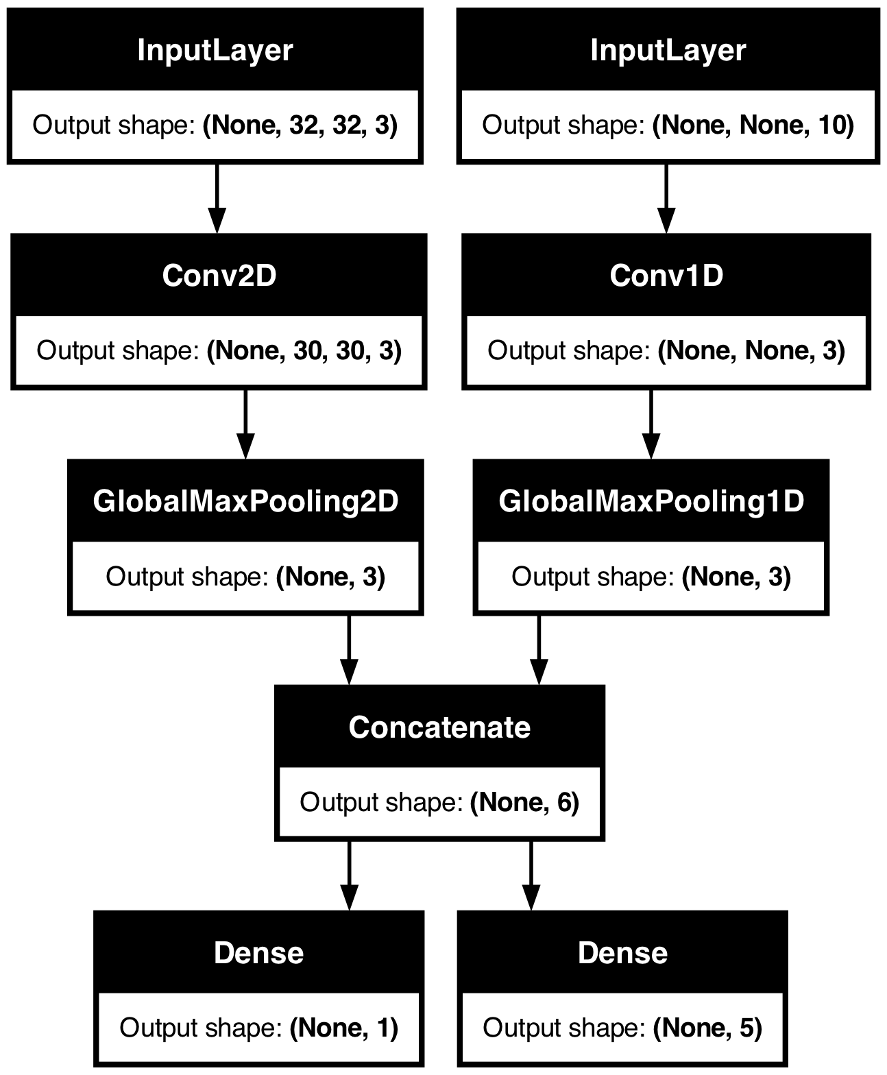
考慮以下模型,它具有形狀為 (32, 32, 3) 的影像輸入(即 (高度、寬度、通道))和形狀為 (None, 10) 的時間序列輸入(即 (時間步長、特徵))。 我們的模型將具有從這些輸入的組合計算出的兩個輸出:「分數」(形狀為 (1,))和五個類別的機率分佈(形狀為 (5,))。
image_input = keras.Input(shape=(32, 32, 3), name="img_input")
timeseries_input = keras.Input(shape=(None, 10), name="ts_input")

x1 = layers.Conv2D(3, 3)(image_input)
x1 = layers.GlobalMaxPooling2D()(x1)

x2 = layers.Conv1D(3, 3)(timeseries_input)
x2 = layers.GlobalMaxPooling1D()(x2)

x = layers.concatenate([x1, x2])

score_output = layers.Dense(1, name="score_output")(x)
class_output = layers.Dense(5, name="class_output")(x)

model = keras.Model(
    inputs=[image_input, timeseries_input], outputs=[score_output, class_output]
)
讓我們繪製這個模型,以便您可以清楚地看到我們在這裡做什麼(請注意,繪圖中顯示的形狀是批次形狀,而不是每個樣本的形狀)。
keras.utils.plot_model(model, "multi_input_and_output_model.png", show_shapes=True)
在編譯時,我們可以透過將損失函數作為清單傳遞,來為不同的輸出指定不同的損失
model.compile(
    optimizer=keras.optimizers.RMSprop(1e-3),
    loss=[
        keras.losses.MeanSquaredError(),
        keras.losses.CategoricalCrossentropy(),
    ],
)
如果我們只將單一損失函數傳遞給模型,則相同的損失函數將應用於每個輸出(這在這裡是不適當的)。
指標也是如此
model.compile(
    optimizer=keras.optimizers.RMSprop(1e-3),
    loss=[
        keras.losses.MeanSquaredError(),
        keras.losses.CategoricalCrossentropy(),
    ],
    metrics=[
        [
            keras.metrics.MeanAbsolutePercentageError(),
            keras.metrics.MeanAbsoluteError(),
        ],
        [keras.metrics.CategoricalAccuracy()],
    ],
)
由於我們為輸出層提供了名稱,我們也可以透過字典指定每個輸出的損失和指標
model.compile(
    optimizer=keras.optimizers.RMSprop(1e-3),
    loss={
        "score_output": keras.losses.MeanSquaredError(),
        "class_output": keras.losses.CategoricalCrossentropy(),
    },
    metrics={
        "score_output": [
            keras.metrics.MeanAbsolutePercentageError(),
            keras.metrics.MeanAbsoluteError(),
        ],
        "class_output": [keras.metrics.CategoricalAccuracy()],
    },
)
如果您有超過 2 個輸出,我們建議使用明確的名稱和字典。
可以使用 loss_weights 參數,為不同的輸出特定損失提供不同的權重(例如,人們可能希望在我們的範例中優先使用「分數」損失,方法是給予類別損失 2 倍的重要性)
model.compile(
    optimizer=keras.optimizers.RMSprop(1e-3),
    loss={
        "score_output": keras.losses.MeanSquaredError(),
        "class_output": keras.losses.CategoricalCrossentropy(),
    },
    metrics={
        "score_output": [
            keras.metrics.MeanAbsolutePercentageError(),
            keras.metrics.MeanAbsoluteError(),
        ],
        "class_output": [keras.metrics.CategoricalAccuracy()],
    },
    loss_weights={"score_output": 2.0, "class_output": 1.0},
)
您也可以選擇不計算某些輸出的損失,如果這些輸出旨在用於預測而不是用於訓練
# List loss version
model.compile(
    optimizer=keras.optimizers.RMSprop(1e-3),
    loss=[None, keras.losses.CategoricalCrossentropy()],
)

# Or dict loss version
model.compile(
    optimizer=keras.optimizers.RMSprop(1e-3),
    loss={"class_output": keras.losses.CategoricalCrossentropy()},
)
在 fit() 中將資料傳遞到多輸入或多輸出模型的工作方式與在編譯中指定損失函數的方式類似:您可以傳遞NumPy 陣列的清單(與接收損失函數的輸出具有 1:1 的對應關係)或將輸出名稱對應到 NumPy 陣列的字典。
model.compile(
    optimizer=keras.optimizers.RMSprop(1e-3),
    loss=[
        keras.losses.MeanSquaredError(),
        keras.losses.CategoricalCrossentropy(),
    ],
)

# Generate dummy NumPy data
img_data = np.random.random_sample(size=(100, 32, 32, 3))
ts_data = np.random.random_sample(size=(100, 20, 10))
score_targets = np.random.random_sample(size=(100, 1))
class_targets = np.random.random_sample(size=(100, 5))

# Fit on lists
model.fit([img_data, ts_data], [score_targets, class_targets], batch_size=32, epochs=1)

# Alternatively, fit on dicts
model.fit(
    {"img_input": img_data, "ts_input": ts_data},
    {"score_output": score_targets, "class_output": class_targets},
    batch_size=32,
    epochs=1,
)
 4/4 ━━━━━━━━━━━━━━━━━━━━ 0s 62ms/step - loss: 18.0146
 4/4 ━━━━━━━━━━━━━━━━━━━━ 0s 56ms/step - loss: 17.6494

<keras.src.callbacks.history.History at 0x31a6c5810>
這是 Dataset 用例:與我們對 NumPy 陣列所做的類似,Dataset 應傳回字典的元組。
train_dataset = tf.data.Dataset.from_tensor_slices(
    (
        {"img_input": img_data, "ts_input": ts_data},
        {"score_output": score_targets, "class_output": class_targets},
    )
)
train_dataset = train_dataset.shuffle(buffer_size=1024).batch(64)

model.fit(train_dataset, epochs=1)
 2/2 ━━━━━━━━━━━━━━━━━━━━ 0s 197ms/step - loss: 17.8578

<keras.src.callbacks.history.History at 0x17c7e5690>
使用回呼
Keras 中的回呼是在訓練期間的不同點(在 epoch 開始時、在批次結束時、在 epoch 結束時等等)呼叫的物件。 它們可用於實作某些行為,例如
- 在訓練期間的不同點進行驗證(超出內建的每個 epoch 驗證)
- 定期或在超過特定準確度閾值時檢查點模型
- 當訓練似乎停滯不前時,變更模型的學習速率
- 當訓練似乎停滯不前時,微調頂層
- 當訓練結束或超過特定效能閾值時,傳送電子郵件或即時訊息通知
- 等等。
回呼可以作為清單傳遞給您對 fit() 的呼叫
model = get_compiled_model()

callbacks = [
    keras.callbacks.EarlyStopping(
        # Stop training when `val_loss` is no longer improving
        monitor="val_loss",
        # "no longer improving" being defined as "no better than 1e-2 less"
        min_delta=1e-2,
        # "no longer improving" being further defined as "for at least 2 epochs"
        patience=2,
        verbose=1,
    )
]
model.fit(
    x_train,
    y_train,
    epochs=20,
    batch_size=64,
    callbacks=callbacks,
    validation_split=0.2,
)
Epoch 1/20
 625/625 ━━━━━━━━━━━━━━━━━━━━ 1s 622us/step - loss: 0.6245 - sparse_categorical_accuracy: 0.8275 - val_loss: 0.2231 - val_sparse_categorical_accuracy: 0.9330
Epoch 2/20
 625/625 ━━━━━━━━━━━━━━━━━━━━ 0s 404us/step - loss: 0.1809 - sparse_categorical_accuracy: 0.9460 - val_loss: 0.1727 - val_sparse_categorical_accuracy: 0.9476
Epoch 3/20
 625/625 ━━━━━━━━━━━━━━━━━━━━ 0s 398us/step - loss: 0.1336 - sparse_categorical_accuracy: 0.9598 - val_loss: 0.1564 - val_sparse_categorical_accuracy: 0.9545
Epoch 4/20
 625/625 ━━━━━━━━━━━━━━━━━━━━ 0s 400us/step - loss: 0.1012 - sparse_categorical_accuracy: 0.9699 - val_loss: 0.1502 - val_sparse_categorical_accuracy: 0.9570
Epoch 5/20
 625/625 ━━━━━━━━━━━━━━━━━━━━ 0s 403us/step - loss: 0.0835 - sparse_categorical_accuracy: 0.9748 - val_loss: 0.1436 - val_sparse_categorical_accuracy: 0.9589
Epoch 6/20
 625/625 ━━━━━━━━━━━━━━━━━━━━ 0s 396us/step - loss: 0.0699 - sparse_categorical_accuracy: 0.9783 - val_loss: 0.1484 - val_sparse_categorical_accuracy: 0.9577
Epoch 7/20
 625/625 ━━━━━━━━━━━━━━━━━━━━ 0s 402us/step - loss: 0.0603 - sparse_categorical_accuracy: 0.9814 - val_loss: 0.1406 - val_sparse_categorical_accuracy: 0.9629
Epoch 7: early stopping

<keras.src.callbacks.history.History at 0x31ae37c10>
提供許多內建回呼
Keras 中已經提供了許多內建回呼,例如
ModelCheckpoint:定期儲存模型。EarlyStopping:當訓練不再改進驗證指標時,停止訓練。TensorBoard:定期寫入可在 TensorBoard 中視覺化的模型日誌(有關更多詳細資訊,請參閱「視覺化」章節)。CSVLogger:將損失和指標資料串流到 CSV 檔案。- 等等。
有關完整清單,請參閱回呼文件。
撰寫您自己的回呼
您可以透過擴展基底類別 keras.callbacks.Callback 來建立自訂回呼。 回呼可以透過類別屬性 self.model 存取其關聯的模型。
請務必閱讀撰寫自訂回呼的完整指南。
這是一個簡單的範例,用於在訓練期間儲存每個批次損失值的清單
class LossHistory(keras.callbacks.Callback):
    def on_train_begin(self, logs):
        self.per_batch_losses = []

    def on_batch_end(self, batch, logs):
        self.per_batch_losses.append(logs.get("loss"))
檢查點模型
當您在相對較大的資料集上訓練模型時,定期儲存模型的檢查點至關重要。
實現此目的的最簡單方法是使用 ModelCheckpoint 回呼
model = get_compiled_model()

callbacks = [
    keras.callbacks.ModelCheckpoint(
        # Path where to save the model
        # The two parameters below mean that we will overwrite
        # the current checkpoint if and only if
        # the `val_loss` score has improved.
        # The saved model name will include the current epoch.
        filepath="mymodel_{epoch}.keras",
        save_best_only=True,  # Only save a model if `val_loss` has improved.
        monitor="val_loss",
        verbose=1,
    )
]
model.fit(
    x_train,
    y_train,
    epochs=2,
    batch_size=64,
    callbacks=callbacks,
    validation_split=0.2,
)
Epoch 1/2
559/625 ━━━━━━━━━━━━━━━━━[37m━━━ 0s 360us/step - loss: 0.6490 - sparse_categorical_accuracy: 0.8209
Epoch 1: val_loss improved from inf to 0.22393, saving model to mymodel_1.keras
625/625 ━━━━━━━━━━━━━━━━━━━━ 1s 577us/step - loss: 0.6194 - sparse_categorical_accuracy: 0.8289 - val_loss: 0.2239 - val_sparse_categorical_accuracy: 0.9340
Epoch 2/2
565/625 ━━━━━━━━━━━━━━━━━━[37m━━ 0s 355us/step - loss: 0.1816 - sparse_categorical_accuracy: 0.9476
Epoch 2: val_loss improved from 0.22393 to 0.16868, saving model to mymodel_2.keras
625/625 ━━━━━━━━━━━━━━━━━━━━ 0s 411us/step - loss: 0.1806 - sparse_categorical_accuracy: 0.9479 - val_loss: 0.1687 - val_sparse_categorical_accuracy: 0.9494
<keras.src.callbacks.history.History at 0x2e5cb7250>
ModelCheckpoint 回呼可用於實作容錯:在訓練隨機中斷的情況下,能夠從模型的最後儲存狀態重新開始訓練。 這是一個基本範例
# Prepare a directory to store all the checkpoints.
checkpoint_dir = "./ckpt"
if not os.path.exists(checkpoint_dir):
    os.makedirs(checkpoint_dir)


def make_or_restore_model():
    # Either restore the latest model, or create a fresh one
    # if there is no checkpoint available.
    checkpoints = [checkpoint_dir + "/" + name for name in os.listdir(checkpoint_dir)]
    if checkpoints:
        latest_checkpoint = max(checkpoints, key=os.path.getctime)
        print("Restoring from", latest_checkpoint)
        return keras.models.load_model(latest_checkpoint)
    print("Creating a new model")
    return get_compiled_model()


model = make_or_restore_model()
callbacks = [
    # This callback saves the model every 100 batches.
    # We include the training loss in the saved model name.
    keras.callbacks.ModelCheckpoint(
        filepath=checkpoint_dir + "/model-loss={loss:.2f}.keras", save_freq=100
    )
]
model.fit(x_train, y_train, epochs=1, callbacks=callbacks)
Creating a new model
 1563/1563 ━━━━━━━━━━━━━━━━━━━━ 1s 390us/step - loss: 0.4910 - sparse_categorical_accuracy: 0.8623

<keras.src.callbacks.history.History at 0x2e5c454e0>
您也可以撰寫自己的回呼來儲存和還原模型。
有關序列化和儲存的完整指南,請參閱模型儲存和序列化指南。
使用學習速率排程
在訓練深度學習模型時,一個常見的模式是隨著訓練的進展逐步降低學習率。這通常被稱為「學習率衰減」。
學習率衰減的排程可以是靜態的(預先固定,作為當前 epoch 或當前批次索引的函數),或動態的(回應模型當前的行為,特別是驗證損失)。
將排程傳遞給優化器
您可以透過將排程物件作為優化器中的 learning_rate 參數傳遞,輕鬆地使用靜態學習率衰減排程。
initial_learning_rate = 0.1
lr_schedule = keras.optimizers.schedules.ExponentialDecay(
    initial_learning_rate, decay_steps=100000, decay_rate=0.96, staircase=True
)

optimizer = keras.optimizers.RMSprop(learning_rate=lr_schedule)
有多種內建排程可供使用:ExponentialDecay、PiecewiseConstantDecay、PolynomialDecay 和 InverseTimeDecay。
使用回呼來實作動態學習率排程
動態學習率排程(例如,當驗證損失不再改善時降低學習率)無法使用這些排程物件實現,因為優化器無法存取驗證指標。
然而,回呼可以存取所有指標,包括驗證指標!因此,您可以透過使用一個回呼來修改優化器上的當前學習率來實現這種模式。事實上,這甚至內建為 ReduceLROnPlateau 回呼。
使用 TensorBoard 在訓練期間視覺化損失和指標
在訓練期間監控模型的最佳方法是使用 TensorBoard – 一個您可以在本地執行的基於瀏覽器的應用程式,它為您提供:
- 訓練和評估的損失和指標的即時圖表
- (可選)您的層激活直方圖的可視化
- (可選)您的
Embedding層學習到的嵌入空間的 3D 可視化
如果您已透過 pip 安裝 TensorFlow,您應該可以從命令列啟動 TensorBoard
tensorboard --logdir=/full_path_to_your_logs
使用 TensorBoard 回呼
將 TensorBoard 與 Keras 模型和 fit() 方法一起使用的最簡單方法是使用 TensorBoard 回呼。
在最簡單的情況下,只需指定您希望回呼寫入日誌的位置,您就可以開始使用了
keras.callbacks.TensorBoard(
    log_dir="/full_path_to_your_logs",
    histogram_freq=0,  # How often to log histogram visualizations
    embeddings_freq=0,  # How often to log embedding visualizations
    update_freq="epoch",
)  # How often to write logs (default: once per epoch)
<keras.src.callbacks.tensorboard.TensorBoard at 0x31b0188b0>
有關更多資訊,請參閱 TensorBoard 回呼的文件。