近乎重複圖片搜尋
作者: Sayak Paul
建立日期 2021/09/10
上次修改日期 2023/08/30

說明: 使用深度學習和局部敏感雜湊建立近乎重複圖片搜尋實用工具。
簡介
在(近乎)即時環境中擷取相似圖片是資訊檢索系統的重要使用案例。一些採用此技術的熱門產品包括 Pinterest、Google 圖片搜尋等。在本範例中,我們將使用局部敏感雜湊 (LSH) 和隨機投影,並以預訓練的圖片分類器計算出的圖片表示為基礎,建立相似圖片搜尋實用工具。這種搜尋引擎也稱為近乎重複 (或近乎重複) 圖片偵測器。我們也將研究如何使用 TensorRT 優化 GPU 上搜尋實用工具的推論效能。
在 keras.io/examples/vision 下方有其他相關的範例,值得查看
最後,此範例使用以下資源作為參考,並因此重複使用其中的一些程式碼:用於相似項目搜尋的局部敏感雜湊。
請注意,為了優化剖析器的效能,您應具有可用的 GPU 執行階段環境。
設定
!pip install tensorrt
匯入
import matplotlib.pyplot as plt
import tensorflow as tf
import tensorrt
import numpy as np
import time

import tensorflow_datasets as tfds

tfds.disable_progress_bar()
載入資料集並建立 1,000 張圖片的訓練集
為了縮短範例的執行時間,我們將使用 tf_flowers 資料集 (可透過 TensorFlow 資料集取得) 中 1,000 張圖片的子集來建立我們的詞彙表。
train_ds, validation_ds = tfds.load(
    "tf_flowers", split=["train[:85%]", "train[85%:]"], as_supervised=True
)

IMAGE_SIZE = 224
NUM_IMAGES = 1000

images = []
labels = []

for (image, label) in train_ds.take(NUM_IMAGES):
    image = tf.image.resize(image, (IMAGE_SIZE, IMAGE_SIZE))
    images.append(image.numpy())
    labels.append(label.numpy())

images = np.array(images)
labels = np.array(labels)
載入預訓練模型
在本節中,我們載入在 tf_flowers 資料集上訓練的影像分類模型。總圖片的 85% 用於建立訓練集。如需更多關於訓練的詳細資訊,請參閱此筆記本。
基礎模型為 BiT-ResNet (在 Big Transfer (BiT):一般視覺表示學習 中提出)。已知 BiT-ResNet 系列模型在各種不同的下游任務中都能提供出色的遷移效能。
!wget -q https://github.com/sayakpaul/near-dup-parser/releases/download/v0.1.0/flower_model_bit_0.96875.zip
!unzip -qq flower_model_bit_0.96875.zip
bit_model = tf.keras.models.load_model("flower_model_bit_0.96875")
bit_model.count_params()
23510597
建立嵌入模型
若要擷取給定查詢圖片的相似圖片,我們需要先產生所有相關圖片的向量表示。我們會透過嵌入模型來執行此操作,該模型會從預訓練的分類器擷取輸出特徵,並將產生的特徵向量正規化。
embedding_model = tf.keras.Sequential(
    [
        tf.keras.layers.Input((IMAGE_SIZE, IMAGE_SIZE, 3)),
        tf.keras.layers.Rescaling(scale=1.0 / 255),
        bit_model.layers[1],
        tf.keras.layers.Normalization(mean=0, variance=1),
    ],
    name="embedding_model",
)

embedding_model.summary()
Model: "embedding_model"
_________________________________________________________________
Layer (type)                 Output Shape              Param #
=================================================================
rescaling (Rescaling)        (None, 224, 224, 3)       0
_________________________________________________________________
keras_layer (KerasLayer)     (None, 2048)              23500352
_________________________________________________________________
normalization (Normalization (None, 2048)              0
=================================================================
Total params: 23,500,352
Trainable params: 23,500,352
Non-trainable params: 0
_________________________________________________________________
請注意模型內部的正規化層。它用於將表示向量投影到單位球體的空間。
雜湊工具
def hash_func(embedding, random_vectors):
    embedding = np.array(embedding)

    # Random projection.
    bools = np.dot(embedding, random_vectors) > 0
    return [bool2int(bool_vec) for bool_vec in bools]


def bool2int(x):
    y = 0
    for i, j in enumerate(x):
        if j:
            y += 1 << i
    return y
從 embedding_model 輸出的向量形狀為 (2048,),且考量到實際層面(儲存、擷取效能等),它相當大。因此,有必要在不減少資訊內容的情況下減少嵌入向量的維度。這就是隨機投影的用武之地。它的基礎原理是,如果給定平面上的一組點之間的距離得到近似保留,則該平面的維度可以進一步減少。
在 hash_func() 內部,我們首先會減少嵌入向量的維度。然後,我們計算圖片的位元雜湊值,以判斷其雜湊儲存區。具有相同雜湊值的圖片很可能會進入相同的雜湊儲存區。從部署的角度來看,位元雜湊值的儲存和運算成本較低。
查詢工具
Table 類別負責建構單一雜湊表。雜湊表中的每個條目都是我們資料集中圖像的降維嵌入與唯一識別碼之間的映射。由於我們的降維技術涉及隨機性,因此相似的圖像在每次執行該過程時可能不會映射到相同的雜湊桶。為了減少這種影響,我們將考慮多個表的結果——表的數量和降維的維度是這裡的關鍵超參數。
至關重要的是,在處理真實世界的應用程式時,您不會自己重新實作局部敏感雜湊。相反,您可能會使用以下其中一個流行的函式庫
class Table:
    def __init__(self, hash_size, dim):
        self.table = {}
        self.hash_size = hash_size
        self.random_vectors = np.random.randn(hash_size, dim).T

    def add(self, id, vectors, label):
        # Create a unique indentifier.
        entry = {"id_label": str(id) + "_" + str(label)}

        # Compute the hash values.
        hashes = hash_func(vectors, self.random_vectors)

        # Add the hash values to the current table.
        for h in hashes:
            if h in self.table:
                self.table[h].append(entry)
            else:
                self.table[h] = [entry]

    def query(self, vectors):
        # Compute hash value for the query vector.
        hashes = hash_func(vectors, self.random_vectors)
        results = []

        # Loop over the query hashes and determine if they exist in
        # the current table.
        for h in hashes:
            if h in self.table:
                results.extend(self.table[h])
        return results
在下面的 LSH 類別中,我們將封裝使用多個雜湊表的工具。
class LSH:
    def __init__(self, hash_size, dim, num_tables):
        self.num_tables = num_tables
        self.tables = []
        for i in range(self.num_tables):
            self.tables.append(Table(hash_size, dim))

    def add(self, id, vectors, label):
        for table in self.tables:
            table.add(id, vectors, label)

    def query(self, vectors):
        results = []
        for table in self.tables:
            results.extend(table.query(vectors))
        return results
現在,我們可以將建構和操作主 LSH 表(多個表的集合)的邏輯封裝在一個類別中。它有兩個方法
train():負責建構最終的 LSH 表。query():計算給定查詢圖像的匹配次數,並量化相似度分數。
class BuildLSHTable:
    def __init__(
        self,
        prediction_model,
        concrete_function=False,
        hash_size=8,
        dim=2048,
        num_tables=10,
    ):
        self.hash_size = hash_size
        self.dim = dim
        self.num_tables = num_tables
        self.lsh = LSH(self.hash_size, self.dim, self.num_tables)

        self.prediction_model = prediction_model
        self.concrete_function = concrete_function

    def train(self, training_files):
        for id, training_file in enumerate(training_files):
            # Unpack the data.
            image, label = training_file
            if len(image.shape) < 4:
                image = image[None, ...]

            # Compute embeddings and update the LSH tables.
            # More on `self.concrete_function()` later.
            if self.concrete_function:
                features = self.prediction_model(tf.constant(image))[
                    "normalization"
                ].numpy()
            else:
                features = self.prediction_model.predict(image)
            self.lsh.add(id, features, label)

    def query(self, image, verbose=True):
        # Compute the embeddings of the query image and fetch the results.
        if len(image.shape) < 4:
            image = image[None, ...]

        if self.concrete_function:
            features = self.prediction_model(tf.constant(image))[
                "normalization"
            ].numpy()
        else:
            features = self.prediction_model.predict(image)

        results = self.lsh.query(features)
        if verbose:
            print("Matches:", len(results))

        # Calculate Jaccard index to quantify the similarity.
        counts = {}
        for r in results:
            if r["id_label"] in counts:
                counts[r["id_label"]] += 1
            else:
                counts[r["id_label"]] = 1
        for k in counts:
            counts[k] = float(counts[k]) / self.dim
        return counts
建立 LSH 表
隨著我們實作的輔助工具和類別,我們現在可以建立我們的 LSH 表。由於我們將基準測試優化和未優化嵌入模型之間的效能,我們也將預熱我們的 GPU 以避免任何不公平的比較。
# Utility to warm up the GPU.
def warmup():
    dummy_sample = tf.ones((1, IMAGE_SIZE, IMAGE_SIZE, 3))
    for _ in range(100):
        _ = embedding_model.predict(dummy_sample)
現在我們可以先執行 GPU 預熱,然後繼續使用 embedding_model 建構主 LSH 表。
warmup()

training_files = zip(images, labels)
lsh_builder = BuildLSHTable(embedding_model)
lsh_builder.train(training_files)
在撰寫本文時,Tesla T4 GPU 的實際時間為 54.1 秒。此時間可能會因您使用的 GPU 而異。
使用 TensorRT 優化模型
對於基於 NVIDIA 的 GPU,TensorRT 架構可透過使用各種模型最佳化技術(例如修剪、常數折疊、層融合等)來大幅提高推論延遲。在這裡,我們將使用 tf.experimental.tensorrt 模組來最佳化我們的嵌入模型。
# First serialize the embedding model as a SavedModel.
embedding_model.save("embedding_model")

# Initialize the conversion parameters.
params = tf.experimental.tensorrt.ConversionParams(
    precision_mode="FP16", maximum_cached_engines=16
)

# Run the conversion.
converter = tf.experimental.tensorrt.Converter(
    input_saved_model_dir="embedding_model", conversion_params=params
)
converter.convert()
converter.save("tensorrt_embedding_model")
WARNING:tensorflow:Compiled the loaded model, but the compiled metrics have yet to be built. `model.compile_metrics` will be empty until you train or evaluate the model.

WARNING:tensorflow:Compiled the loaded model, but the compiled metrics have yet to be built. `model.compile_metrics` will be empty until you train or evaluate the model.

INFO:tensorflow:Assets written to: embedding_model/assets

INFO:tensorflow:Assets written to: embedding_model/assets

INFO:tensorflow:Linked TensorRT version: (0, 0, 0)

INFO:tensorflow:Linked TensorRT version: (0, 0, 0)

INFO:tensorflow:Loaded TensorRT version: (0, 0, 0)

INFO:tensorflow:Loaded TensorRT version: (0, 0, 0)

INFO:tensorflow:Assets written to: tensorrt_embedding_model/assets

INFO:tensorflow:Assets written to: tensorrt_embedding_model/assets
關於 tf.experimental.tensorrt.ConversionParams() 內參數的注意事項:
precision_mode定義要轉換的模型中運算的數值精度。maximum_cached_engines指定將快取以處理動態運算(具有未知形狀的運算)的 TRT 引擎的最大數量。
要了解有關其他選項的更多資訊,請參閱官方文件。您還可以探索 tf.experimental.tensorrt 模組提供的不同量化選項。
# Load the converted model.
root = tf.saved_model.load("tensorrt_embedding_model")
trt_model_function = root.signatures["serving_default"]
使用最佳化模型建立 LSH 表
warmup()

training_files = zip(images, labels)
lsh_builder_trt = BuildLSHTable(trt_model_function, concrete_function=True)
lsh_builder_trt.train(training_files)
請注意實際時間的差異,它是 13.1 秒。先前,使用未最佳化的模型是 54.1 秒。
我們可以仔細研究其中一個雜湊表,並了解它們的表示方式。
idx = 0
for hash, entry in lsh_builder_trt.lsh.tables[0].table.items():
    if idx == 5:
        break
    if len(entry) < 5:
        print(hash, entry)
        idx += 1
145 [{'id_label': '3_4'}, {'id_label': '727_3'}]
5 [{'id_label': '12_4'}]
128 [{'id_label': '30_2'}, {'id_label': '480_2'}]
208 [{'id_label': '34_2'}, {'id_label': '132_2'}, {'id_label': '984_2'}]
188 [{'id_label': '42_0'}, {'id_label': '135_3'}, {'id_label': '436_3'}, {'id_label': '670_3'}]
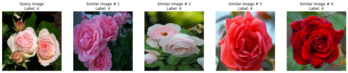
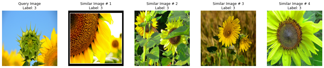
視覺化驗證圖像的結果
在本節中,我們將首先編寫幾個輔助函式,以視覺化相似圖像的剖析過程。然後,我們將基準測試具有和不具有最佳化的模型之查詢效能。
首先,我們從驗證集中取出 100 張圖像用於測試目的。
validation_images = []
validation_labels = []

for image, label in validation_ds.take(100):
    image = tf.image.resize(image, (224, 224))
    validation_images.append(image.numpy())
    validation_labels.append(label.numpy())

validation_images = np.array(validation_images)
validation_labels = np.array(validation_labels)
validation_images.shape, validation_labels.shape
((100, 224, 224, 3), (100,))
現在我們編寫我們的視覺化工具。
def plot_images(images, labels):
    plt.figure(figsize=(20, 10))
    columns = 5
    for (i, image) in enumerate(images):
        ax = plt.subplot(len(images) // columns + 1, columns, i + 1)
        if i == 0:
            ax.set_title("Query Image\n" + "Label: {}".format(labels[i]))
        else:
            ax.set_title("Similar Image # " + str(i) + "\nLabel: {}".format(labels[i]))
        plt.imshow(image.astype("int"))
        plt.axis("off")


def visualize_lsh(lsh_class):
    idx = np.random.choice(len(validation_images))
    image = validation_images[idx]
    label = validation_labels[idx]
    results = lsh_class.query(image)

    candidates = []
    labels = []
    overlaps = []

    for idx, r in enumerate(sorted(results, key=results.get, reverse=True)):
        if idx == 4:
            break
        image_id, label = r.split("_")[0], r.split("_")[1]
        candidates.append(images[int(image_id)])
        labels.append(label)
        overlaps.append(results[r])

    candidates.insert(0, image)
    labels.insert(0, label)

    plot_images(candidates, labels)
非 TRT 模型
for _ in range(5):
    visualize_lsh(lsh_builder)

visualize_lsh(lsh_builder)
Matches: 507
Matches: 554
Matches: 438
Matches: 370
Matches: 407
Matches: 306
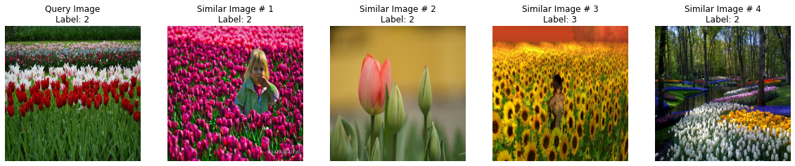
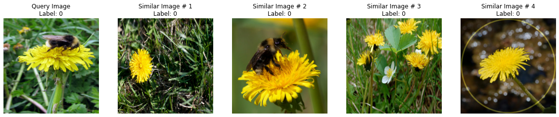
TRT 模型
for _ in range(5):
    visualize_lsh(lsh_builder_trt)
Matches: 458
Matches: 181
Matches: 280
Matches: 280
Matches: 503
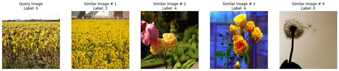

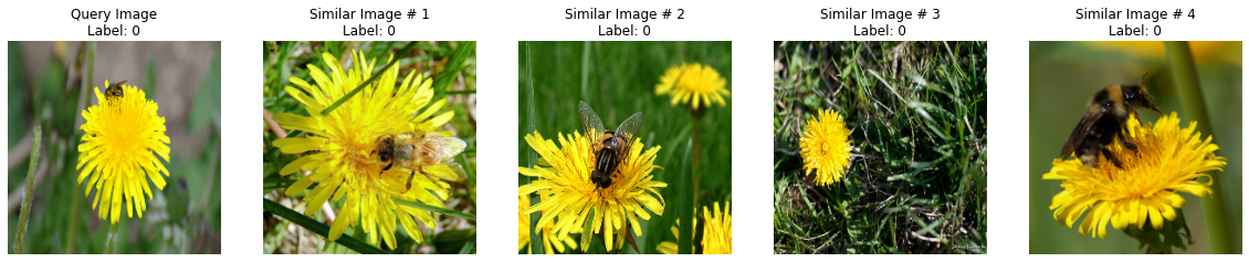
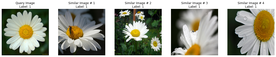
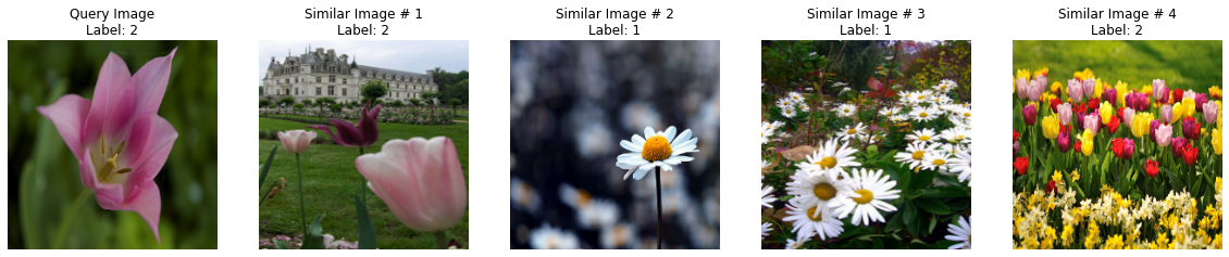
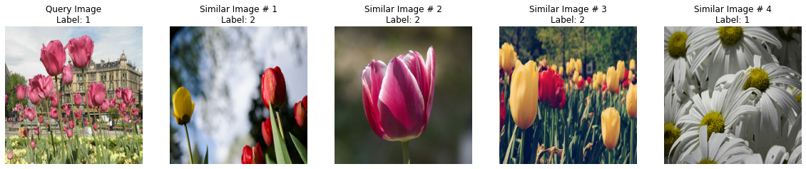
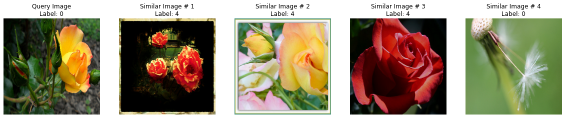
您可能已經注意到,有一些不正確的結果。這可以透過幾種方式來緩解
- 更好的模型用於產生初始嵌入,尤其適用於雜訊樣本。我們可以使用諸如 ArcFace、監督式對比學習等技術,這些技術隱式地鼓勵更好地學習用於檢索目的的表示。
- 表數量與降維之間的權衡至關重要,有助於設定您的應用程式所需的正確召回率。
基準測試查詢效能
def benchmark(lsh_class):
    warmup()

    start_time = time.time()
    for _ in range(1000):
        image = np.ones((1, 224, 224, 3)).astype("float32")
        _ = lsh_class.query(image, verbose=False)
    end_time = time.time() - start_time
    print(f"Time taken: {end_time:.3f}")


benchmark(lsh_builder)

benchmark(lsh_builder_trt)
Time taken: 54.359
Time taken: 13.963
我們可以立即注意到這兩個模型的查詢效能之間存在顯著差異。
總結
在這個範例中,我們探索了 NVIDIA 的 TensorRT 架構來最佳化我們的模型。它最適合基於 GPU 的推論伺服器。對於此類架構,還有其他選項適用於不同的硬體平台
- TensorFlow Lite 用於行動和邊緣裝置。
- ONNX 用於商品化的基於 CPU 的伺服器。
- Apache TVM,用於機器學習模型的編譯器,涵蓋各種平台。
以下是一些您可能想要查看的資源,以了解有關一般基於向量相似度搜尋之應用程式的更多資訊